Variance And Bias

by Matthew Baas

This aims to explain my understanding of what people refer to when they talk bias and variance in the context of a function approximator.

UPDATE June 2020: After having progressed a bit more in my studies and reflecting on this post, it would seem that it is truly an introductory view that does not contain all the nuance required for the topic – it could definitely be expanded more. Please read the article as a true first-time introduction to the statistical notion of variance and bias and not a detailed deep-dive.

TL;DR What is bias and variance with reference to a function approximator?

Variance (of a function approximator) is a measure of the variability of the output of the approximator relative to the expectation of its output.

Bias (of a function approximator) is a measure of the constant offset of the expected output of some function approximator and the true output value of function it is approximating.

In more detail:

Bias and variance can mean many things, even in deep learning there is a distinction in meaning in different contexts. For example, the ‘bias’ in “the dataset has a bias toward …” entails something different than the ‘bias’ in “adding this term to the loss reduces its bias”. Here we shall make it concrete and only explore what bias and variance are when referring to some function approximator (like the ‘bias’ in the second example).

Often in deep learning we use some function approximator in our models – from the value function estimation \(V(s)\) used in reinforcement learning to the output logit that a certain image is a cat in a classification model. Neural networks are actually just rather effective function approximators. So in deep learning when people refer to the ‘bias’ or ‘variance’ of a model, they are usually referring to that model’s function approximator.

The math

In general, if we have some function approximator \(f(x)\) which attempts to approximate an unknown function \(F(x)\) we can define the bias and variance.

Given a set of \(n\) samples of \(f(x)\), the variance of \(f\) is:

\[var(f) = \frac{1}{n-1}\sum_{i=1}^n(f(x_i)- \mathrm E[f(x)])^2\]

The expected value is usually calculated from the mean of the \(n\) input-output pairs.

For a single input \(x\), the bias of \(f\) is:

\[\mathrm{Bias}(f) = \mathrm E[f(x)] - F(x)\]

For multiple data points, where we have \(n\) tuples of \((x, f(x), F(x))\) we can also get an indication of the average bias by taking the average of the above formula over all the given data points.

Ideally if we are aiming to approximate a function perfectly we want the bias to be 0 and the variance to be small. Practically however, there is often a trade-off between low-bias and low-variance. Techniques which lower the bias usually tend to increase variance, and many techniques which lower variance increase the bias.

Remarks

For the following suppose we have a simple function \(F(x) = log(x)\) and now we are given a model (a function approximator) \(f(x)=log(x)+ some\ noise\) and we want to visualize the bias and variance of \(f\) in its estimation of \(F\).

1. The problem with high variance is that we require many samples with the model to obtain an accurate value for the function.

i.e more samples are needed for the mean of the samples to approach the expectation. Consider the following plots of \(F(x) = log(x)\) (the true function) and \(f(x)=log(x) + scaled\ uniform\ noise\) with a differing number of samples for each input value:

datapoints = []
for i in range(1, 40):
	samples = []
	for j in range(n_samples):
		samples.append(np.log(i) + scale*np.random.uniform(-1, 1))
	datapoints.append(samples)

We can then plot the estimator’s output (in blue) vs the true function’s output (in green) for various values of scale (which scales the random noise added) and n_samples (how many times to sample the estimator for each input), which gives us the figure below. The light blue filled region gives an indication of the variance of function at the current input. The figure shows several plots of the estimator (blue) and true function (green) for various values of \(x\). From left to right, the amount of uniform noise used in the estimator decreases, while from top to bottom the amount of samples per data point increases (as labeled on top of each plot).

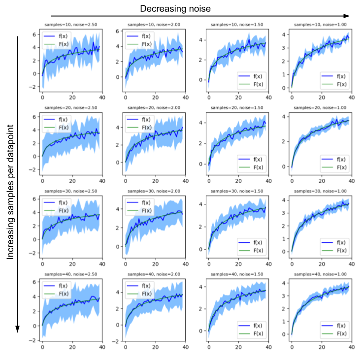
We can see the effect of the number of samples and noise scale with the accuracy of our estimator. For a constant number of samples, decreasing noise scale directly means decreasing variance (and thus making our estimator more accurate). For A constant noise level, more samples gives a more accurate (mean) value estimate for the target function. Also see the illustration of point 1: the higher the noise, the more samples we need to get an accurate value (blue line) for the target function (green line).

Side note: ideally we want to be in the bottom right corner, with lots of samples and low noise. In reality, however, the sampling action is usually expensive (e.g simulating games of Dota 2) and decreasing noise often comes with increasing bias. It is a design trade-off where on this plot you have the resources to operate.

2. High bias is not necessarily a problem.

It depends on what you want to do and how you want to try achieve it. It can be quite bad if, for example, we make a reinforcement learning agent with a value function approximator (like a big neural net) which consistently underestimates its value when it takes some game-winning position. This might lead to inaccurate or dysfunctional planning or control. On the other hand if we train a neural net to predict future stock prices, we might actually want to enforce some downward of the future price approximator so that you are always on the cautious side with your money.

3. Sampling more does not allow you to alter the effects of bias.

Because function approximator / model bias compares the expectation of the approximator to the true function, only the true mean of the approximator defines the bias. So the noise and sampling does not change the effects of bias.

To visualize this, have a look at the set of plots below where again we plot (in green) \(F(x) = log(x)\) and now, holding the noise and number of samples constant, plot (in blue) \(f(x) = k\cdot log(x) + scaled\ noise\) for varying values of bias scaling \(k\) (bias_scale in the code/figure).

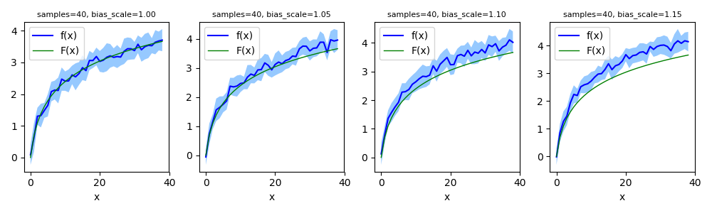
It is pretty clear: the noise and number of samples will not change the bias.

4. Function approximators can have differing bias and variance characteristics over differing regions of their domain.

As was hinted in 2, a function approximator could very well have high variance/bias for some \(x\) and low variance/bias for others. For example, a reinforcement learning agent might reliably take a decision during one part of a game but be wildly uncertain during other parts. Often however, the bias and variance characteristics are very similar over large parts of the domain.

5. Many things in deep learning can be phrased as function approximation.

Although here I only looked concretely at bias and variance for function approximation, many parts of deep learning can be phrased as function approximation. For example:

• Stochastic gradient descent approximates the gradient function by using only a few samples to estimate a gradient.
• The \(Q_{\theta}(s, a)\) function parameterized by some big neural net in Q-learning approximates the true action-value function.
• The discriminator in vanilla GAN’s are a function approximator of the indicator function flagging genuine and counterfeit inputs.

I hope that the above was succinct and helpful. If I have made an error, especially in the math, please do get in contact so it can be corrected.

Thanks!