M Baas
I am a machine learning researcher at Camb.AI. I post about deep learning, electronics, and other things I find interesting.
Basic X-ray powder diffraction with fastai
by Matthew Baas
Performing simple X-ray diffraction (XRD) classification with convolutional neural networks.
This post will explain how to do XRD classification for simple cases with convolutional networks and fastai. The aim is to be succinct while giving enough explanation that would still make it easy to implement the general method on new problems.
Background: at a recent hackathon at Stellenbosch University, one problem was to classify simple XRD measurement samples (the XRD data was provided by Nanodyn, so super thanks to them). So, here I explain my entry to do this using pytorch and fastai to do it with neural networks.
As with most deep learning problems, we need 3 things:
- Data
- Loss
- Model
1. Data
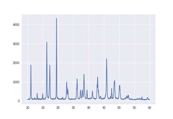
We are given 92 X-ray diffraction measurements, with each measurement being one of 5 different types of crystals and some being labelled as anomalies. So after parsing the format of these XRD measurements, each one looks like the image below. Essentially we treat each XRD as a vector of numbers \(x\), treating it similar to a time-series. Keeping things extremely general so as to not use any domain knowledge of XRD, what the x and y axis represent for each XRD measurement is not labelled and we don’t learn about them (in fact we actually discard the x-axis in the image below, since we can treat the y-values as a 1D time series and the plot would look the same).
Each XRD sample is labelled as being of crystal A, B, C, D, E or an anomaly. Now since we will use a convolutional network to classify them, it makes sense to maybe try and change the appearance of these graphs or array of numbers into something more visual. If we find a way to do this nicely, we can perform lots of all the image transforms usually used for visual data (cropping, zooming, adjusting contrast…) on this 1D vector of numbers.
Now a cool recent idea for doing this is to apply a Gramian angular field, which basically takes in a 1D array of numbers and spits out a grayscale image. It may seem weird to apply a transform usually reserved for time series to XRD data which is not a function of time, but it still effectively transforms a 1D array of numbers into a picture in a sensible way, so why not use it. The details of the transform are not too important, and can be easily applied to an XRD sample with the pyts python package:
import pyts.image
X_gadf = pyts.image.gaf.GramianAngularField(256, method='difference')
# x here is a numpy array of the XRD measurement.
# E.g shape for x is (23140,), and in the above image each value in x is roughly between 0-4200
x = x.reshape(1, *x.shape) # puts x into shape needed by pyts
lol = X_gadf.transform(x)
plt.imshow(lol.squeeze(), cmap='viridis')
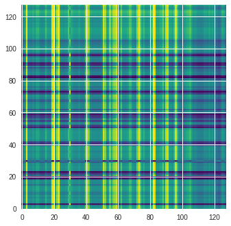
This changes the above image into a picture like the one below. Note how we used the viridis colormap to map the grayscale image to a color one. This is not critical, but fastai has very good native support for 3-channel RGB images so it makes the coding a bit more seamless.
Ok cool all set – we now have 92 pairs of (image, crystal type). We save the images to a folder ./data/ and the labels into a csv labels.csv.
Getting data ready for training
Now we need to apply transforms, group data into minibatches, make a validation and training set, normalize data… The great news is fastai makes all this super easy:
from fastai import *
from fastai.vision import *

path = './data/'
# now get all the transforms we want to apply. Do not flip or rotate them since
# if you look at the Garmian angular field you can see flipping it or rotating
# it drastically changes its meaning.
tfms = get_transforms(do_flip=False, max_rotate=0.0, max_zoom=1.08, max_warp=0.01)

data = (ImageList.from_csv('./', 'labels.csv', folder='data')
        .split_by_rand_pct(valid_pct=0.15) # optionally you can specify a random seed
        .label_from_df(label_cls=CategoryList)
        .transform(tfms, size=128)
        .databunch()
        .normalize(imagenet_stats))
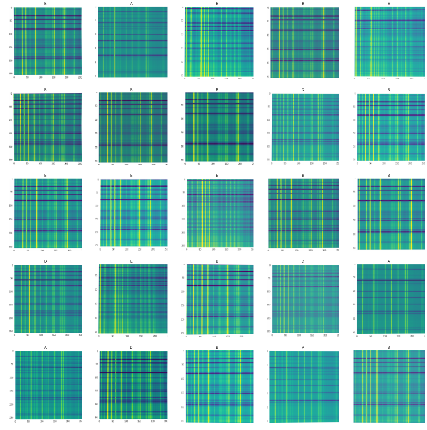
Done! This data object is used by fastai when training the neural network. It generates batches, applies transforms and handles all the tricky bits of making a proper dataset. A batch of data now looks like:
2. Loss
Since the task is a common one of single-class classification, fastai takes care of this and makes the model’s loss function the categorical cross-entropy loss usually used for classification. It knew to use the usual classification loss since when we defined data we labelled the images with a CategoryList.
3. Model
The simplest way to create a good CNN in fastai is to use a Resnet model pretrained on ImageNet and then retrain on our data. And to train we need to specify a learning rate for the neural network. A good pick for the learning rate can be found with the lr_find() method:
learn = cnn_learner(data, models.resnet34, metrics=accuracy) # use a pretrained Resnet34 model
learn.lr_find()
learn.recorder.plot()
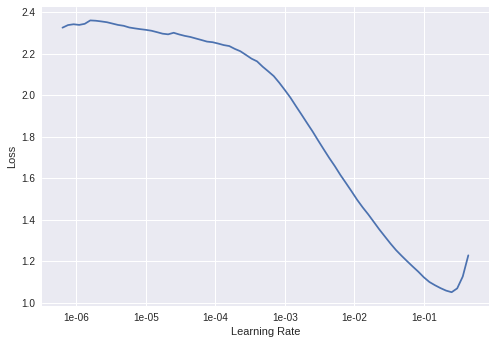
This created a resnet of 34 layers pretrained to recognize various everyday objects in ImageNet. The learning rate finder gives the plot below, and as is the method we pick a learning rate near where the gradient is the largest and while the learning rate is still as quite large – 2e-2 seems like a good bet.
Now we just train the network for a few epochs. The first few trains only the new final, untrained layer of the resnet model while all the earlier layers are kept ‘frozen’ and the training does not modify their weights.
learn.fit_one_cycle(4, 2e-2)
| epoch | train_loss | valid_loss | accuracy | time |
|---|---|---|---|---|
| 0 | 2.342362 | 1.587954 | 0.437500 | 00:02 |
| 1 | 2.131937 | 1.423728 | 0.687500 | 00:01 |
| 2 | 1.620610 | 1.452918 | 0.687500 | 00:01 |
| 3 | 1.295927 | 1.584721 | 0.687500 | 00:01 |
There we go – already at 68.75% accuracy after about 8 seconds of training. Now that the last layer is reasonably good (read: now has trained weights which make the accuracy pretty good), we unfreeze the weights of the rest of the network and re-run the learning rate finder, and train some more. The code to do this is only a few lines:
learn.unfreeze()
learn.lr_find()
learn.recorder.plot() # run the lr finder again
The new learning rate finder produces the plot below. Now, since the earlier layers of the pretrained network are probably already have quite good weights for most tasks (e.g edge detection, contrasts…) so we apply a lower learning rate to the earlier layers and a bigger one to the later layers.
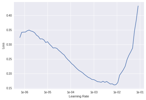
Again from the plot we make the biggest learning rate 1e-4 (for the final layers) and the smallest 5e-4 (for the first several layers).
Fastai then makes the learning rates of the layers between the first and last to vary between these two bounds.
learn.fit_one_cycle(10, slice(5e-4, 1e-4))
| epoch | train_loss | valid_loss | accuracy | time |
|---|---|---|---|---|
| 0 | 0.345086 | 1.439965 | 0.687500 | 00:01 |
| 1 | 0.330607 | 1.144911 | 0.750000 | 00:01 |
| 2 | 0.303133 | 0.930825 | 0.687500 | 00:01 |
| 3 | 0.283710 | 0.592039 | 0.875000 | 00:01 |
| 4 | 0.265402 | 0.521643 | 0.937500 | 00:01 |
| 5 | 0.251848 | 0.466204 | 0.937500 | 00:01 |
| 6 | 0.244248 | 0.419879 | 0.937500 | 00:01 |
| 7 | 0.228994 | 0.340093 | 0.937500 | 00:01 |
| 8 | 0.215688 | 0.250459 | 0.937500 | 00:01 |
| 9 | 0.202289 | 0.191805 | 0.937500 | 00:01 |
This gives us a solid 93.75% accuracy, which is only 1 image wrong with a 18% validation set and 92 images. Done after in total ~20 seconds of training :).
Looking at results
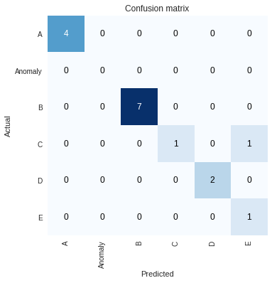
We can look at a confusion matrix of the results very easily as well:
preds,y,losses = learn.get_preds(ds_type=DatasetType.Valid, with_loss=True)
interp = ClassificationInterpretation(learn, preds, y, losses)
interp.plot_confusion_matrix()
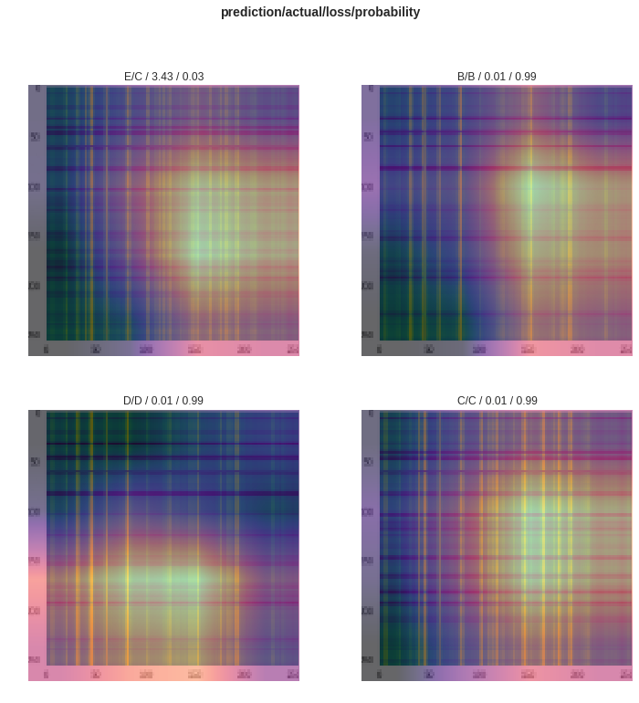
Another very interesting insight is to see where the activations are on the images with the highest loss (including the single failure case), which we can find with interp.plot_top_losses(4), giving the image below where brighter means the neural network activations were larger for those parts of the image near the final layers. Although not too informative for these Gramian transformed images, often it can be cool to see where the network is looking to make its decision.
So we got a pretty nice accuracy with a pretty modern network in very few lines and with only 92 data samples. This process was also super generic, having nothing problem-specific to XRD, except perhaps the Gramian transform which is specific to 1D time-series like data. So nearly the exact same code can be applied to many other classification problems with good-to-great success.
A final note is that the XRD data used for this little task is of mostly single crystal samples, and that full XRD analysis is significantly more complicated. This just showed that in the simple case it is fairly straightforward to make a CNN with pytorch & fastai to classify an XRD as one of a few crystals with not too many data samples.
tags: deep learning - fastai - pytorch - XRD