Basic antenna parameters - A quick reference

by Matthew Baas

A quick rundown of the basic antenna parameters, in the notation used at Stellenbosch University.

TL;DR: After a few courses in electromagnetics, and an introduction to antenna theory, the core parameters that characterize an antenna seem really important, yet after a while I found myself forgetting what they meant a little. And when searching online, the notation is everywhere, and a lot of stuff is not general but contains many situation-specific clauses in their definitions or equations.

So, I aim to give a quick overview of basic antenna parameters, using the notation which I found to work very well – that is, the notation used by the Stellenbosch University electromagnetics department. This post assumes the reader has knowledge of a few basic electromagnetics courses, and it is intended to be a quick reference for definitions and equations in the notation used at Stellenbosch.

Basic antenna definitions

Electromagnetic notation basics

• Cartesian coordinates parameterized by \(x, y, z\).
• Spherical coordinates parameterized by \(r, \theta, \phi\).
• The propagation constant is \(\gamma = \alpha + j \beta\). For the most part in this, we neglect losses in the medium (i.e the attenuation constant \(\alpha = 0\)), and approximate the medium with \(\beta = \omega \sqrt{\mu \epsilon}\). Usually \(\mu = \mu_0\), \(\epsilon = \epsilon_0 \epsilon_r\) for relative permittivity \(\epsilon_r\). I will try to make it clear if I rely on this assumption, and keep its use to a minimum.
• We will focus our analysis and parameterize things in terms of the electric field intensity \(\vec{E}\), and magnetic field intensity \(\vec{H}\).
• All field variables \(\vec{E}, \vec{H}\) denote phasor fields. Since we mostly denote time-harmonic phasor fields, assume all denotations of field quantities are phasors unless explicitly indicated otherwise. That is, to indicate a time-domain quantity I will explicitly show the time dependence. i.e \(\vec{E}(x, y, z) = \vec{E}\) denotes a phasor quantity, while \(\vec{E}(x, y, z, t) = \vec{E}(t)\) denotes a time-domain quantity.
• The current is denoted \(I\), while the current (surface/volume/line) density is denoted \(\vec{J}\).
• Sometimes vector fields (which have an x, y, z component in Cartesian coordinates) are denoted with a vector arrow above the variable (used here), or by emboldening the variable. That is, \(\vec{E} = \mathbf{E} = E_x \mathbf{a_x} + E_y \mathbf{a_y} + E_z \mathbf{a_z}\) for unit vectors \(\mathbf{a_x}, \mathbf{a_y}, \mathbf{a_z}\) in the +x, +y, and +z direction, respectively.

The Hertzian Dipole

The ideal/Hertzian/elemental dipole is the simplest radiative element studied as the basis for more complex antenna constructions. It is defined as a line (electric) current in a wire of infinitesimal length and diameter. Using a standard Cartesian coordinate system, a Hertzian dipole at the origin is depicted as:

The E and H field of such an element contains terms proportional to \(\frac{1}{r}\), \(\frac{1}{r^2}\), and \(\frac{1}{r^3}\). The expression for E and H (i.t.o spherical coordinates) for most antenna structures and arrays are comprised of terms proportional to \(\frac{1}{r^n}\) for small integer \(n\). In the figure, note that the current density is related to the current by \(I=|\vec{J}| \pi d\rho\) for infinitesimal radius \(d\rho\) for \(\rho\) in cylindrical coordinates.

Near-field

Near-field is the region ‘close’ to the antenna (array) structure. Exactly how close is not set in stone, but in general it is close enough such that the expression for the E and H field may be approximated with only the term inversely proportional to highest power of \(r\) (\(\frac{1}{r^n}\)), and the terms proportional to lower powers of \(r\) are neglected. In such cases the E and H field vectors are perpendicular to one another but not necessarily perpendicular to the direction of propagation.

Far-field

Far-field, conversely, is the region ‘far away’ from the antenna (array) structure. Exactly how far is not set in stone, but in general it is far enough such that the expression for the E and H field may be approximated with only the term proportional to \(\frac{1}{r}\), and the higher order terms can be neglected. In such cases the E and H field vectors are perpendicular to one another and perpendicular to the direction of propagation of the wave.

Usually the near-field quantities are harder to analyze than the far-field quantities because of complex interactions near the surface of antenna structures. There are some expressions one can use to judge whether the far- or near-field approximations are appropriate at a given radius \(r\).

Antenna parameters

1. Radiation patterns and plots

1.1 Definition: Radiation pattern

The radiation pattern of an antenna is defined as the magnitude/absolute value of the portion of the E (or H) field’s dependence on \(\theta\) and \(\phi\) in the far-field region. Concretely, in the far-field region, the E (and H) field will always be expressible as:

For some function \(F\) dependent on only \(\theta\) and \(\phi\). The expression \(|F(\theta, \phi)|\) is defined as the radiation pattern of the antenna. For the Hertzian dipole, this is equal to \(|\sin(\theta)|\).

1.2 Plotting radiation patterns

To plot the radiation pattern \(|F(\theta, \phi)|\) with \(\theta\) and \(\phi\) as independent variables, and \(F(\theta, \phi)\) as the dependent variable, we can either use cartesian coordinates, or polar coordinates. The two kinds of plots for the Hertzian dipole are shown below:

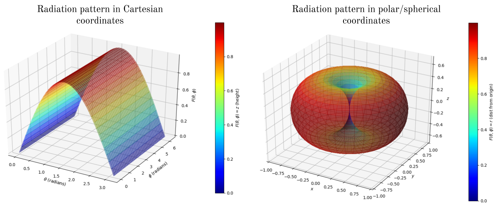
In the Cartesian plot, the height \(z\) is the dependent parameter, while in the polar/spherical plot the radius \(r\) is the dependent parameter. Both kinds of plots are used, however usually to simplify things we only plot 2D slices of such 3D plots. The 2D slices through certain planes are of special importance, discussed next.

1.3 Definition: The H-plane

The H-plane is that plane in the current coordinate system which is perpendicular to the antenna current vector \(\vec{J}\). Usually this is also the plane containing the far-field \(\vec{H}\) vector. The H and E plane are generally used to construct univariate graphs of the E-field or \(F\) i.t.o either \(\phi\) or \(\theta\).

For a z-oriented dipole, this is the xy plane. So, if we were to plot \(F\) (or |E| or |H|, for that matter) in the H-plane for the Hertzian dipole, it would be a straight horizontal line i.t.o \(\phi\). Since in the H plane, the only variable that changes in the spherical coordinate system is \(\phi\), and from the 3D polar plot in the above image, you can see that the xy plane intersects the surface at a constant radius from the origin (and thus constant \(F\), since that is how 3D polar plots are defined).

1.4 Definition: The E-plane

Conversely, the E-plane is that plane containing the antenna current vector \(\vec{J}\). Usually this is the plane containing the vector \(\vec{E}\) and contains the direction of maximum radiated E-field. For the Hertzian dipole (with +z directed current as shown earlier), this is any plane with constant \(\phi\) (that is, any plane perpendicular to the xy plane).

The E and H planes are always perpendicular to one another. For the Hertzian dipole, if we were to plot \(F(\theta, \phi)\) (or |E|, |H|) vs \(\theta\) (since the radiation pattern only depends on \(\theta, \phi\), and the E-plane by definition is for a constant \(\phi\)), then we would see the plot of \(|\sin(\theta)|\) vs \(\theta\). Note how to visualize this from looking at the 3D polar plot of the Hertzian dipole above.

As an example, consider a linear array of 4 Hertzian dipoles along the \(x\)-axis, with \(+z\) directed currents, as shown in the image below.

In the image, I also show the H and E planes. Recall that in general the E and H planes are not unique, however for the antenna array setup shown, the only plane which acts as an E plane for all the antenna elements is the xz-plane. For a single dipole element, the H and E plane could be chosen as long as they conform to their definitions.

2. Power parameters

First, recall that the Poynting vector is defined as:

It is the vector of instantaneous power propagation. However, this is an instantaneous quantity, and to use the phasor domain we need to express the E and H fields as phasors, in which case the instantaneous value is of no use. Thus, when dealing with phasors and antennas, we work with the time average power \(\vec{P}_{avg}\) (of some time-harmonic electric and magnetic fields). That is,

Which can be shown, using the definition of the Poynting vector, to simplify when E and H are sinusoidal phasor fields to:

That is, half of the real part of the E phasor crossed with the conjugate of the H-field phasor. This \(\vec{P}_{avg}\) is known as the time-average Poynting vector (aka power intensity) (aka ‘complex Poynting vector’, which is a weird thing to call it since it is by definition real, but eh I didn’t make these names). For many antenna structures, this power radiates radially outward from the antenna structure, thus if the antenna structure is placed at the origin then usually \(\vec{P}_{avg}\) direction is radially outward.

2.1 Definition: Total radiated power

Using this time-average Poynting vector, which is the average outward power intensity at every point in space due to the antenna currents, we can find the total radiated power by just integrating over a spherical surface far away from the antenna. That is, we define the total radiated power, \(P_r\) as:

Where \(\mathbf{\vec{a}_r}\) is the unit vector in the radially outward direction (assuming the antenna is centered at the origin). Note that the power intensity, total radiated power I define here are only for far-fields. That is, the E and H fields used to compute \(\vec{P}_{avg}\) should be the far-fields. Note: the surface is definitely a closed sphere, however the closed surface integral symbol is not supported by MathJax (what this website uses to render math), so rip. Secondly, note that \(\vec{P}_{avg}\) should be dependent on \(\frac{1}{r^2}\), since in the far-field both the E and H vectors are proportional to \(\frac{1}{r}\). And since the surface of a sphere grows proportional to \(r^2\), it is also always true that the total radiated power equation above should simplify to a constant (with respect to radius) once the integral has been evaluated.

2.2 Definition: Radiation intensity

The radiation intensity of an antenna is the power radiated per unit solid angle, with solid angles in Steradians. It is given the symbol \(U(\theta, \phi)\) and is in general dependent on \(\phi\) and \(\theta\) (but not the radius). Concretely, it is defined as:

Again, this only applied to far-field analysis. Note: the area on a spherical surface of radius \(r\) in 1 steradian is \(r^2\).

2.3 Definition: Input power

The input power \(P_i\) is defined as the total power available to the antenna, at the antenna terminals (i.e after some of the source power has been reflected due to impedance mismatches along the transmission line). The total radiated power and input power are related by: \(P_r = P_i - P_l\) Where \(P_l\) is the total power losses due to non-ideal effects (like power loss due to conductor resistance or a non-zero attenuation constant).

3. Gains and Directivity

All the following parameters pertain to the far-field behavior of a particular antenna element.

3.1 Definition: Directive gain

The directive gain \(G_D (\theta, \phi)\) is the ratio of the magnitude of the power intensity (aka time-average Poynting vector) at a particular \(\theta, phi\) to the power intensity of a fictitious antenna element that radiated the same total power as the antenna in question, but does so isotropically (read: the same in all directions radially). That is,

Since this is a ratio, it is dimensionless. Expressed another way, the directive gain is the ratio [power intensity at some \(\theta, \phi\)]/[the average power intensity at any \(\theta, \phi\) of some fictitious antenna that has the same total radiated power as the original antenna and dissipates that power isotropically]. This parameter is one of the more important ones for characterizing antenna elements. It is often expressed in terms of decibels (dB), and since it is already a power ratio, to convert the numerical value of \(G_D\) to dB, simply go \(10\log(G_D)\).

3.2 Definition: Directivity

The directivity of an antenna, \(D\), is the maximum directive gain. That is,

This gives an indication of how well the antenna can focus its radiated power in some direction. The higher \(D\), the more the antenna can direct its radiated far-fields to some receiver. Note this is not to be confused with directive gain, however in some texts just calling something ‘directivity’ sometimes actually refers to the directive gain.

3.3 Definition: Power gain

The power gain \(G_p (\theta, \phi)\) is the ratio of the magnitude of the power intensity (aka time-average Poynting vector) at a particular \(\theta, phi\) to the power intensity of a fictitious antenna element that radiated the same input power as the antenna in question, but does so isotropically. That is,

Note the power gain is sometimes just called the ‘gain’ of the antenna. The only difference between the power gain and directive gain is that the power gain is normalized with the input power supplied to the antenna. Thus \(G_p\) is usually a bit lower than \(G_D\) since the total radiated power is less than the total input power because of losses. Again, both \(G_p\) and \(D\) are often expressed in decibels.

There is another gain called the realized gain, which normalizes not with the radiated or input power, but with the actual source power that feeds the transmission line into the antenna. This is again even lower than the power gain because the input power to the antenna is the source power less the power lost over the transmission line due to slightly lossy media.

3.4 Definition: Radiation efficiency

The radiation efficiency is simply the ratio of radiated power to input power. That is, \(\eta_r = \frac{P_r}{P_i} = \frac{G_p}{D} \le 1\)

4. Resistance and length

Two more parameters that are often used to characterize an antenna are the radiation resistance and effective length.

4.1 Definition: Radiation resistance

The radiation resistance is that value of resistor, such that if the same current \(I\) that flows in the antenna, flows in the resistor, the antenna will have the same total radiated power as the Ohmic power dissipated in the resistor. That is,

Where \(R_r\) is the radiation resistance in Ohms, and \(I\) is the current flowing in the antenna element. This is essentially an ‘equivalent resistance’ for the antenna, and can be used to help match transmission lines. A separate resistance value can be found for the power losses \(P_l\) as \(R_l\) using a similar procedure. The antenna can then be modelled as the radiation resistance in series with \(R_l\).

4.2 Definition: Effective length

The effective length of an antenna is that length \(l_e\) of constant (phasor) magnitude line current that radiates the same (far-field) E-field magnitude as the original antenna in the direction where the original antenna’s maximum radiation pattern occurs when the line current magnitude is the same as the maximum current in the original antenna. That is, given the generic far-field \(\vec{E}_{\text{line}}\) of a line current, how long must that line current be such that it has the same magnitude in the direction where the original antenna had a maximum magnitude. From some math we can show

(Don’t worry too much about the symbols and notation for \(\vec{E}_{\text{line}}\)). Then if the antenna under question has the E-field expression given by \(\vec{E}\), then finding the effective length is done by setting:

And solving for \(l_e\). This is often dependent on the frequency of radiation.

5. Radiation beams and shapes

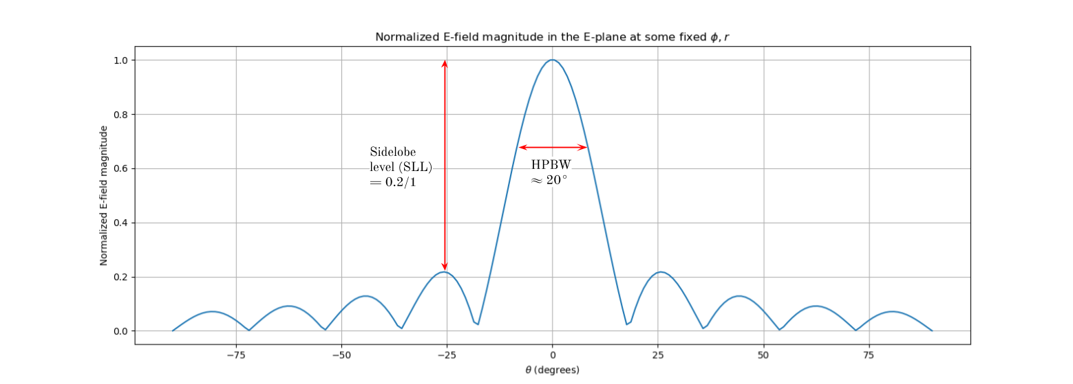
The actual shape of the radiation patterns are classified in terms of a few parameters. Usually if we plot radiation patterns in the E-plane (either Cartesian coordinates \(|\vec{E}|\) vs \(\theta\) as y and x, or polar with \(|\vec{E}|\) vs \(\theta\) as r and \(\theta\)), then we observe several maxima and minima of E-field magnitudes. For example, here is a rough diagram of a kind of shapes we would expect to see, from Wikipedia:

This is a polar plot of the E-field magnitude in the E-plane for some moderately complex antenna. Each region between two minima in the radiation pattern / E-field magnitude is called a radiation lobe.

5.1 Definition: Main lobe

The main lobe is that radiation lobe centered around the direction of maximum E-field magnitude / maximum radiation pattern \(F(\theta, \phi)\).

5.2 Definition: Side lobes

Side lobes are in general all radiation lobes which are not the main lobe. The back lobe is sometimes included in the side-lobes.

5.3 Definition: Beamwidth

The beamwidth of an antenna is the angular size of the main lobe. It is usually quantified with the variable in 5.4.

5.4 Definition: Half-power beamwidth

The half-power beamwidth (HPBW) is the beamwidth measured as the angle (in degrees or radians) between the two points in the main lobe where the power intensity/directive gain has dropped to half of its maximum. Or equivalently, where the E-field magnitude or the radiation pattern have dropped to a factor of \(\frac{1}{\sqrt{2}}\) of their maximum in the main lobe.

For the Hertzian dipole, this is 90 degrees.

5.5 Definition: Sidelobe level

The sidelobe level (SLL) is the ratio of the electric field magnitudes between the first (and largest) sidelobe maximum to the maximum electric field magnitude of the main lobe. This is usually expressed in dB. As an example of calculating the SLL and HPBW, see below a Cartesian plot of the normalized E-field magnitude (same shape as radiation pattern \(|F(\theta, \phi)|\)) vs \(\theta\) in some E-plane for some antenna element.

Last comments

Antenna arrays have even more terminology and parameters, however I don’t know enough to give a confident reference for that just yet. PS: if you think I’ve got something wrong, please let me know (leave a message in the ‘About’ section).

Super thanks to the great electromagnetics lecturers in the E&E department at Stellenbosch, they really helped me understand the content well (together with Field and Wave Electromagnetics by Cheng, however that is quite a dry read).

Anyway, I hope this was a bit useful, or at the very least looked cool. Have a good day.