A simple 2D STFT module in pytorch

by Matthew Baas

This post aims to provide a simple, efficient, and differentiable 2D STFT module in pytorch.

TL;DR: In digital signals processing, the discrete fourier transform (DFT) is a mainstay of analysis and modelling of many systems. For signals that vary with time, such as audio, the short-time Fourier transform (STFT) is often useful to see how the frequency content of the signal changes over time.

The STFT is often used in machine learning and audio processing in particular, where it is useful that this STFT representation can be computed in both a rapid and differentiable way. These systems are typically one-dimensional, however both the DFT and STFT can generalize to multiple dimensions. I could not find a ready-to-use differentiable 2D STFT, so I made one, and present it briefly here. This post assumes basic knowledge of the 1D FFT and how it works.

If you only care about the code, click here.

1. Motivation

The 1D STFT (what most people are referring to when talking about an ‘STFT’) is well-known and widely used, with extremely performant and feature-rich implementations in both pytorch, librosa, and other libraries.

These are used overwhelmingly for audio, mostly to mel-scaled spectrograms or for loss components in certain vocoders such as vocos. The robustness and feature richness of the common STFT implementations in libraries have, I believe, largely enabled many of these applications, and the progress in speech processing would be much slower without them.

Now, on the other side of the kinds of signals humans can experience are images. Images are 2D and vary in both an ‘x’ and a ‘y’ direction. So, the question arises: what about 2D DFT and STFT modules? Where are they? Could they be of similar widespread use for image processing applications?

Looking into this, I found two things:

• For 2D DFTs, they exist fine and well, with performant and feature-rich implementations in torch, numpy, and all other kinds of libraries.
• For 2D STFTs, I could not find any that were (a) fast/performant, and (b) differentiable.

So, I decided to make one as a fun exercise. For this implementation, I will not be focused too much on the theoretical math, but instead will keep things short and simple by focusing on the implementation details. The goal here is to make a 2D STFT torch.nn module which:

• Is fast: vectorized, runs on the GPU, and is batched
• Is differentiable: allows gradients to propagate through it accurately
• Is correct: actually a correct 2D STFT implementation and not just the input signal times 10.

For the theory behind this work, I will largely be drawing on lectures presented by Prof Herman Kamper and Prof Thomas Niesler at Stellenbosch University.

2. Method

The development goes like this:

1. In 1D, we have a continuous signal and sample it. This sampling action is equivalent to duplicating the frequency spectrum of the signal at the sampling frequency.
2. In 2D, we have a continuous signal, and sample it using a 2D grid of sampling points (e.g. pixel coordinates) at a rate of $f_x$ and $f_y$ for x and y coordinates. This is equivalent to duplicating the frequency spectrum at all integer multiples of $f_x$ and $f_y$. So sampling in the time/space domain again leads to periodicity in the frequency domain, either 1D or 2D periodicity.
3. The DFT/FFT in 1D is obtained by taking the discrete Fourier transform of the 1D signal in question. E.g. a discrete time signal of $N$ samples will be mapped to a frequency spectrum of $N$ frequencies. However, for most real signals of interest, the samples beyond $N/2$ will be a mirror image of those up to $N/2$ due to the spectrum duplication of discrete-time signals
4. Similarly, the 2D DFT/FFT is obtained by taking the discrete Fourier transform in 2D (i.e. a 2D FFT). E.g. a discrete image signal of $N_x$ by $N_y$ samples will be mapped to a frequency spectrum of $N_x$ by $N_y$ frequencies. However, for most real signals of interest, the samples beyond $N_x/2$ and $N_y/2$ will be a mirror image of those up to $N_x/2$ and $N_y/2$ due to the spectrum duplication of discrete-time signals.
5. For taking the 1D STFT, we do a vectorized implementation of the following:

output_frames = [] # empty list
window_tensor = window_function(window_length)

for i in range(0, N, hop_length):
    windowed_frames = signal[i:i*window_length] * window_tensor
    fft_coeffs = fft(windowed_frames) # a 1D signal
    output_frames.append(fft_coeffs)

output_frames = torch.stack(output_frames) # stacked 1D signals, i.e. a 2D signal

1. Phrased in this way, it is easy to see how to generalize this to 2D:

output_frames = [] 
window_tensor = window_function_2d(window_length_x, window_length_y)

for x in range(0, N_x, hop_length_x):
    output_row = []
    for y in range(0, N_y, hop_length_y):
        windowed_image = signal[x:x+window_length_x, y:y+window_length_y] * window_tensor
        fft_coeffs = fft_2d(windowed_image) # a 2D signal
        output_row.append(fft_coeffs)
    
    output_frames.append(output_row) # list of 2D signals, i.e. a 3D signal

output_frames = torch.stack(output_frames) # stacked 3D signals, i.e. a 4D signal. 

All that is left is to convert the above for-loop-based pseudocode into vectorized form. And, as it turns out, LLMs are pretty good at that if you help them along and give them the right docs, namely torch.unfold and torch.reshape docs. A similar process of reasoning can be applied to inverse transform, and then again optimized with the help of autocomplete models. One caveat in my implementation is that I use separable 2D windows only , and not perfect symmetrical 2D windows. However, the code is simple enough to allow for your own modifications, and I expect most machine learning models would be able to adapt to most common kinds of window functions you throw at it.

After the base implementation, all that is left is testing and edge case fixing (like padding the edges of an image, handling batches/multi-channel inputs, and singleton dimensions). The end result is two functions with the following signatures:

class STFT2D(nn.Module):

    def __init__(self, win_len=(64, 64), win_hop=(32, 32), fft_len=(64, 64),
                 win_type='hann', pad_center=True):
        """
        2D Short-Time Fourier Transform (STFT) module for multi-channel images.

        The parameters win_len, win_hop, fft_len are tuples (value_for_width, value_for_height).

        Args:
            win_len (tuple of int): Window lengths for width and height dimensions. (len_w, len_h).
                                    Defaults to (64, 64).
            win_hop (tuple of int): Hop lengths for width and height dimensions. (hop_w, hop_h).
                                    Defaults to (32, 32).
            fft_len (tuple of int): FFT lengths for width and height dimensions. (fft_w, fft_h).
                                    Should be >= win_len. Defaults to (64, 64).
            win_type (str): Type of window to use (e.g., 'hann', 'hamming'). Passed to scipy.signal.get_window.
                            Defaults to 'hann'.
            pad_center (bool): If True, pads the input signal so that frames are centered.
                               Important for perfect reconstruction. Defaults to True.
        """
        ...

    def transform(self, inputs: torch.Tensor) -> torch.Tensor:
        """
        Performs 2D STFT on multi-channel images.
        Input H, W order is maintained for freq and frame count output dimensions.

        Args:
            inputs (torch.Tensor): Input tensor of shape (H, W), (C, H, W), or (N, C, H, W).
                                   H is height, W is width, N is the batch size, and C is num channels.
        Returns:
            torch.Tensor: STFT coefficients of shape 
                          (N, C, num_freqs_H, num_freqs_W, num_frames_H, num_frames_W).
                          num_freqs_H = fft_len_h // 2 + 1 (from rfft2 on H-dim of patch)
                          num_freqs_W = fft_len_w (from rfft2 on W-dim of patch)
                          num_frames_H = number of frames extracted along the H dimension.
                          num_frames_W = number of frames extracted along the W dimension.
        """
        ...

    def inverse(self, stft_coeffs_user: torch.Tensor) -> torch.Tensor:
        """
        Performs 2D inverse STFT for multi-channel STFT coefficients.
        Expects coeff order (N, C, freq_H, freq_W, frames_H, frames_W).
        Args:
            stft_coeffs_user (torch.Tensor): STFT coefficients of shape 
                                 (N, C, num_freqs_H, num_freqs_W, num_frames_H, num_frames_W) or
                                 (C, num_freqs_H, num_freqs_W, num_frames_H, num_frames_W).
        Returns:
            torch.Tensor: Reconstructed signal, shape matching original input to transform (e.g. (N,C,H,W)).
        """
        ...

To give a concrete example, an RGB image of 1024x1536 pixels will be a tensor of shape (1, 3, 1024, 1536). If we use that with the 2D STFT implementation above, and use a 32x32 window, with a 16x16 pixel hop length, we will obtain an output of shape (1, 3, 17, 32, 65, 97). These numbers may seem initially puzzling, but each can be explained in turn:

• The first dimension is the batch dimension. It’s only a single image, so only 1 in both of them.
• The second dimension is the channel dimension. The STFT is computed separately for each channel as though it were a separate image. Hence both are 3.
• The third and fourth dimensions are the actual 2D FFT frequency bins, and correspond to the window size used. Since we used a 32x32 window, we might expect the output to be 32x32. However, remember that half the frequencies for real signals are duplicates by their symmetry property, so we only need to keep half of the non-zero frequencies, which is (32/2) + 1 = 17, where the 1 is added for the DC/zero-frequency term. This leaves us with 17x32. An equivalent implementation could also take the other dimension of frequencies to half, i.e. it could have used (32, 17) instead.
• The last two dimensions are the spatial dimensions, akin to the time axis on an STFT. These index the patch of the image we are looking at for each 2D FFT. With a hop length of 16x16 pixels, we’d expect $1024/16 = 64.0$, $1536/16 = 96.0$. This is slightly smaller than our outputs above. However, the default arguments in the STFT module above have pad_center=True, which pads the signal by half a hop length on all four sides of the image, effectively extending both dimensions by a full hop length, and therefore making the output spatial shape (65, 97).

Nice and simple when taken one dimension at a time, right?

3. Examples

Here I will walk through a basic example. For ease of visualization, here I will mostly use black and white images (i.e. images with a single channel), as otherwise it becomes harder to visualize the effects.

First, we initialize the transform and image:

from stft2dlib import STFT2D

# initialize the transform
n_fft = window_len = 32
hop_len = 16
tfm = STFT2D(win_len=(window_len, window_len), win_hop=(hop_len, hop_len), fft_len=(n_fft, n_fft))

# load the image
from PIL import Image
image = Image.open("my_file.jpg")

# convert to greyscale tensor
import torchvision
to_tensor = torchvision.transforms.PILToTensor()
im = to_tensor(image) / 255
to_greyscale = torchvision.transforms.Grayscale()
im = to_greyscale(im)
print(im.shape) # torch.Size([736, 981]), floats between 0 and 1

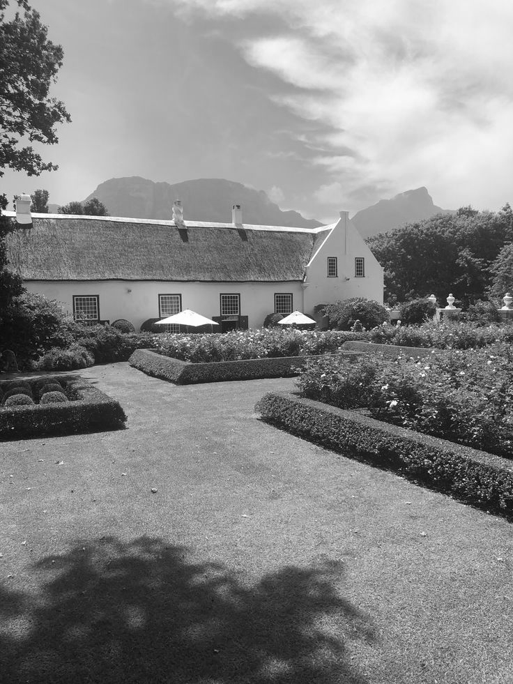
Example 3.1: a photograph

As a first example, let’s consider the following photo of a house in the Cape:

Continuing the above code, we can now get the 2D STFT and its inverse:

im_stft = tf.transform(im[None]) # torch.Size([1, 1, 17, 32, 62, 47]), complex dtype
im_reconstructed = tf.inverse(im_stft) # torch.Size([1, 1, 981, 736])

To gain a better idea of what this information represents, let’s plot along some axes. Like 1D STFTs, the data is actually complex. So, to make it simpler to plot, we look only at the log magnitude: im_stft_db = im_stft.abs().clamp(min=1e-5).log() . Like with audio spectrogram data, for typical images this means that the magnitudes lie roughly between -12 and 2, with most centered around -5.

To gain a first idea, let’s first look at the x-axis / vertical frequencies. That is, we’re going to slice into num_freqs_W dim of the 2D STFT, where each slide is going to correspond to a fixed value of y/horizontal frequency. Concretely, below I am plotting the zeroth y/horizontal frequency: im_stft[0, 0, i, 0] where I am varying i in each subplot. I.e. each subplot is showing a different x/vertical frequency:

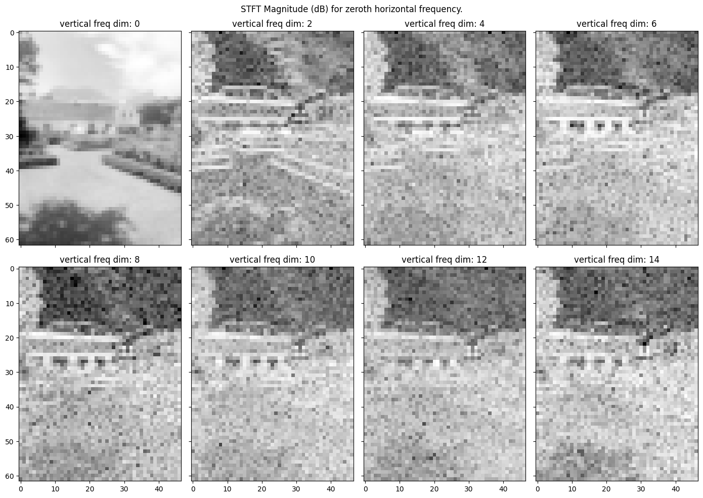
One can see the expected result: the zeroth x-frequency looks basically like a low-resolution version of the image; this is effectively the DC/average component of each 32x32 image patch, given our 32x32 window size. As we increase x/vertical frequencies in the other subplots, we see the contrast emphasize differences in pixel intensities when moving vertically. This is particularly pronounced at the boundary of the house and background, as well as the black windows on the white walls. For very high frequencies, only those frequencies corresponding to the sudden black/white intensity switch around the window borders play a role, as well as the house top outline. The key thing to note is the presence of these horizontal lines – this makes sense since the pixel intensity change over the vertical axis is the same for most pixels e.g. along the roof edge of the house.

Next, let’s look at the horizontal frequencies. For this, I will only look at the zeroth x/vertical frequency, i.e. im_stft[0, 0, 0, i] for each subplot i:

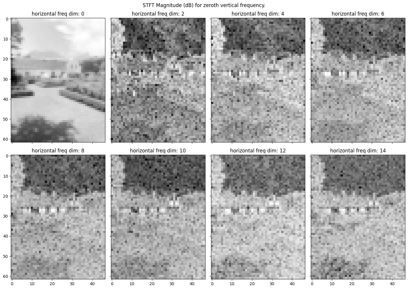
Here we see a similar but slightly different pattern. Here, the strongest patterns we see are the horizontal lines corresponding to places where the horizontal pixel variations are the same for a range of vertical pixels. The two prime examples of this in the image are (1) the tree on the left-hand side, and (2) the vertical edges of the windows on the house and, to a lesser extent, the two chimneys on the house.

The other slices corresponding to intermediate frequencies are a little harder to interpret, e.g. the 2D magnitude plot corresponding to im_stft[0, 0, 8, 15] isn’t entirely clear what it represents, although it’s clear it is some combination of x and y variation that plays into it. Finally, we can plot the reconstructed image from the 2D ISTFT:

Nifty! And gradients flow through the STFT function nicely! So feel free to go wild with using this to train things that need gradients or otherwise batched GPU computation. For reference, here is the full-color version:

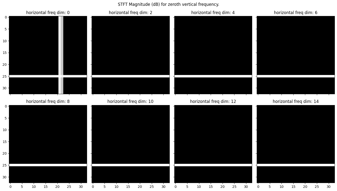
Example 3.2: simplified line image

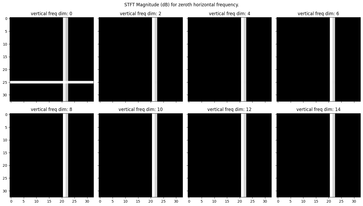
To gain a better understanding of what each slice of this 4-axis tensor looks like, let us consider the following toy image, which is black everywhere save for a single vertical and horizontal white line:

We can repeat the above and again plot the various vertical frequencies for the zeroth horizontal frequency in the first plot, and similarly plot the various horizontal frequencies for the zeroth vertical frequency in a second plot. In the below plots, the hop and window lengths are the same as in the prior example.

Predicting which lines will be present vs not is not entirely intuitive, however, there are some good interactive toys online to get a better feeling for what each frequency bin represents, such as this one. For example, if we plot the 2D STFT of not the zeroth, but instead the 4th horizontal frequency for varying vertical frequencies, the plot now looks like:

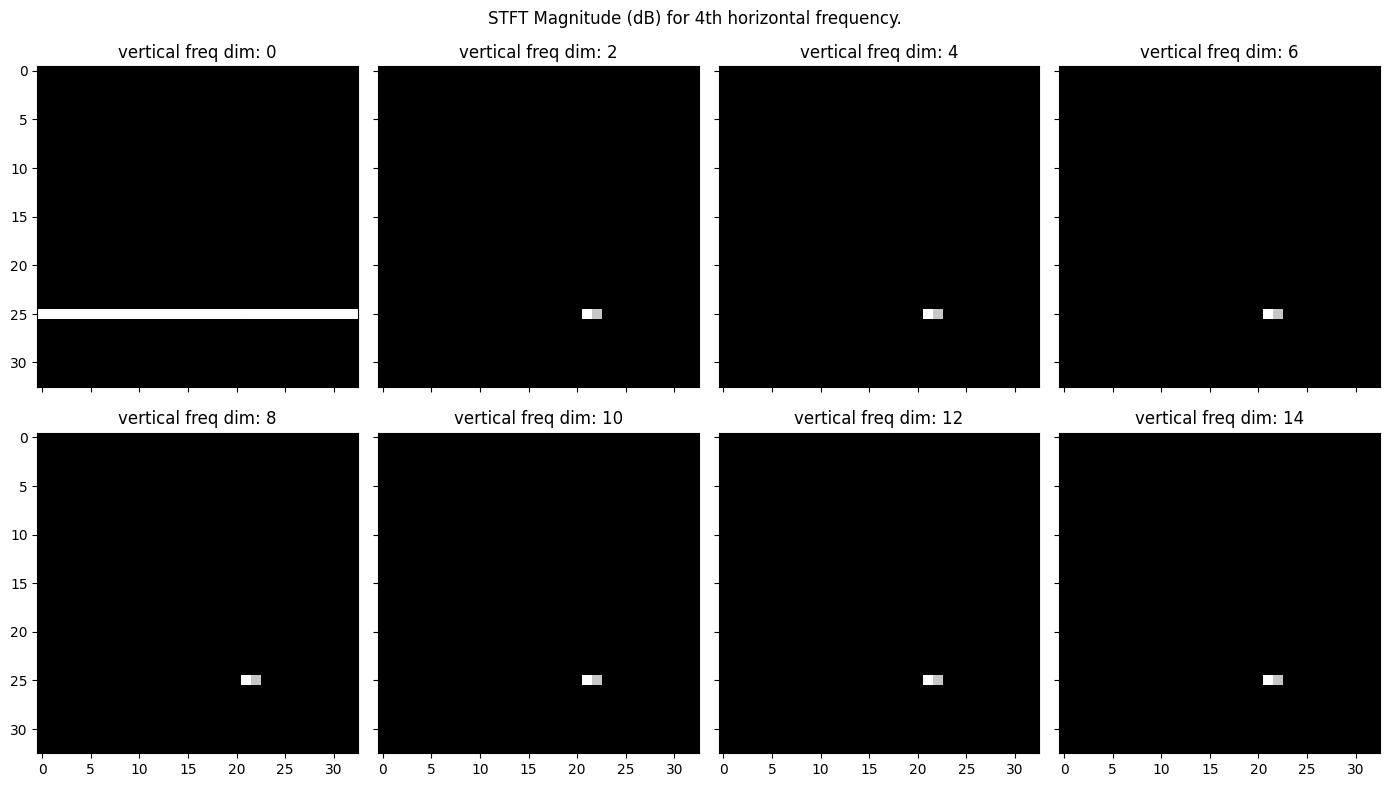
Where now only the intersection of the two lines has non-zero magnitudes for non-zero vertical frequency. There are a few good resources on the theory and reasoning as to why these particular slices should appear like this (like the toy above, or this video), and I’d encourage interested readers to seek them out, or just play with the code to get a more hands-on experience.

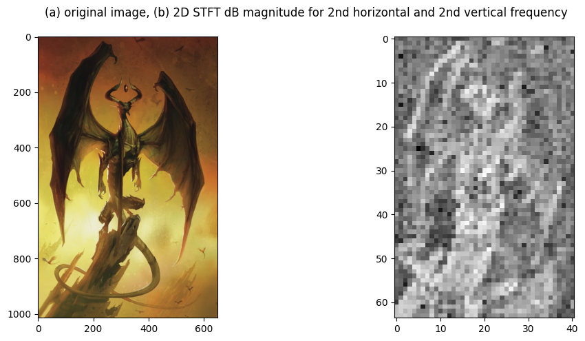
Example 3.3: An RGB image

As a last fun example, here is an RGB image of a dragon, as well as the STFT for the 2nd horizontal and vertical frequency of the red channel:

5. Summary

This post was fairly short compared to prior ones, and addresses the simple problem: I could not find an existing implementation of a 2D STFT out there that was (a) performant and robust, and (b) differentiable.

So, I set out to make a simple implementation of a 2D STFT that supports batching, gradient computation, multi-channel inputs, and is fairly easy to customize if one so wishes. Please, feel free to use the code if you so desire: github link. If you use it, an acknowledgement would be nice though :).

If you spot any mistakes or have any comments in general, feel free to get in touch with me via the about page.

And as always, thank you for reading!