GAN You Hear Me?
Reclaiming unconditional speech synthesis from diffusion models
Demo website for the submitted paper to SLT 2022
Introduction
This is the demonstration website for the paper submitted for SLT 2022. It contains generated audio samples from both our ASGAN model and the baseline implementations against which we compare.
Code & Pretrained models
Please find the quickstart inference and training code on our github repo and the pretrained models on the releases tab of the github repo.
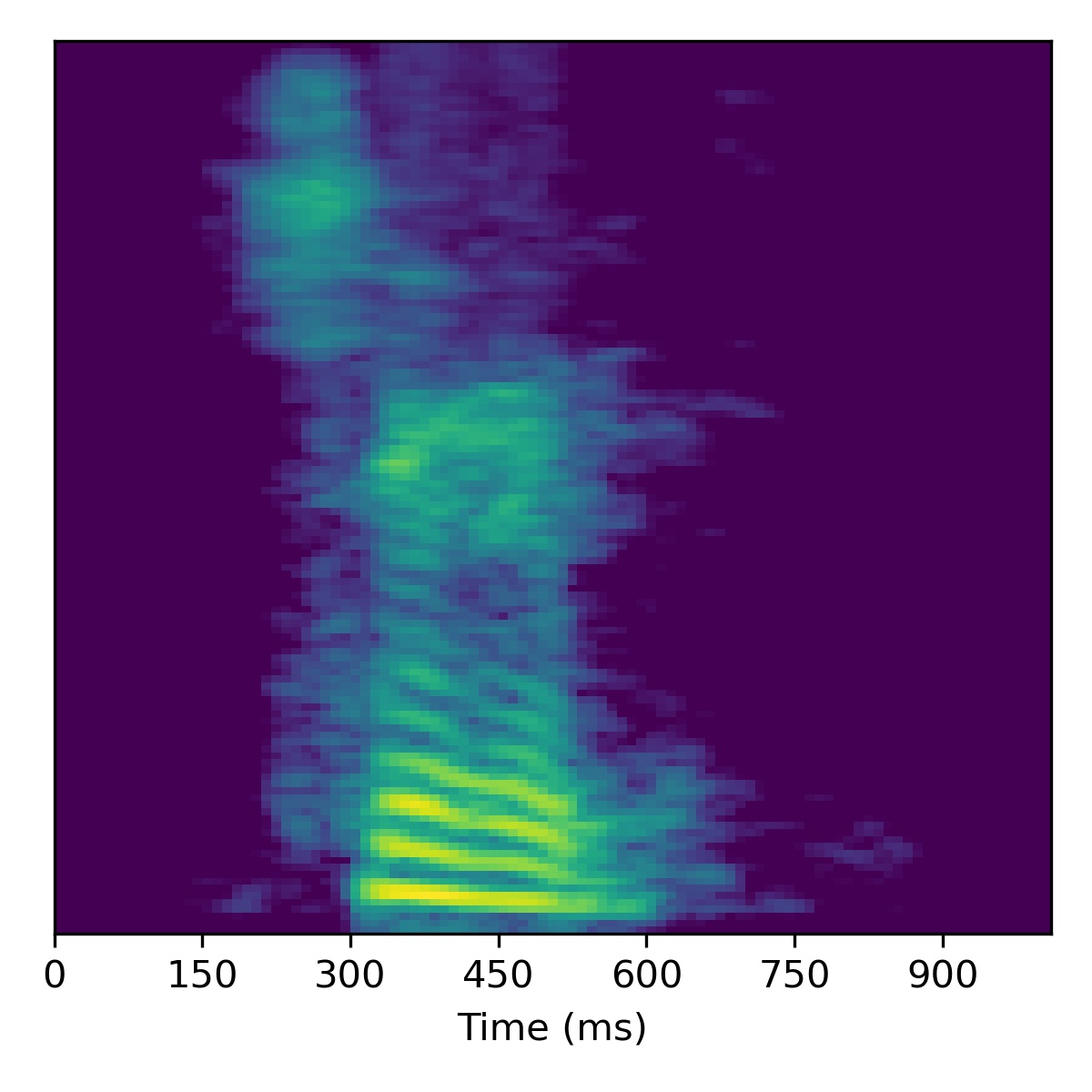
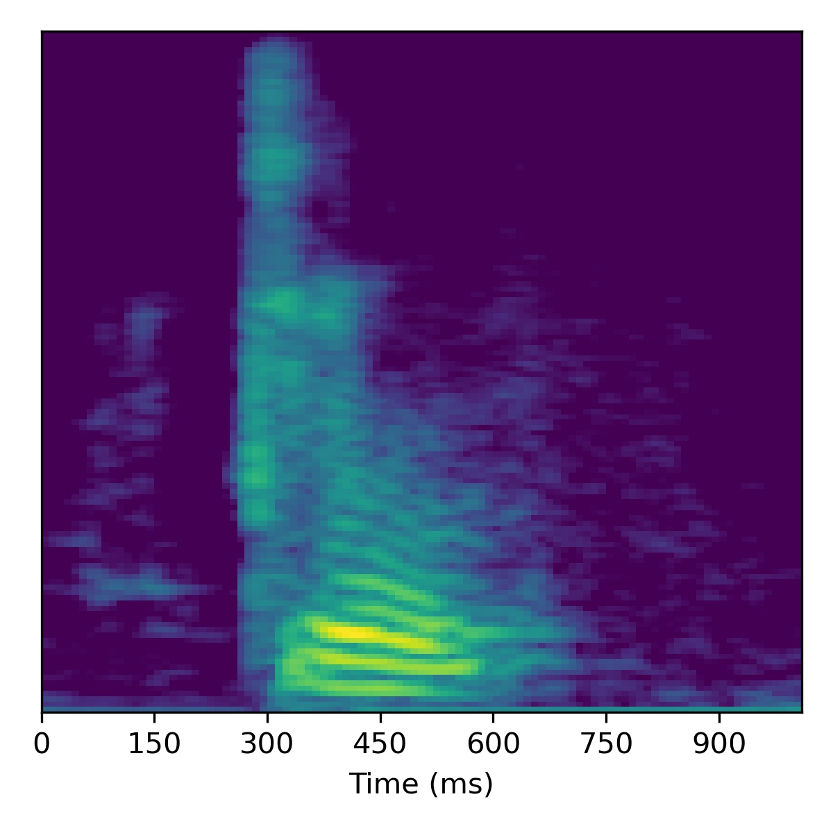
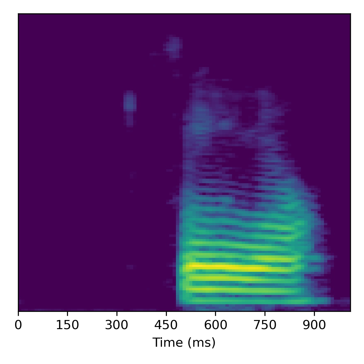
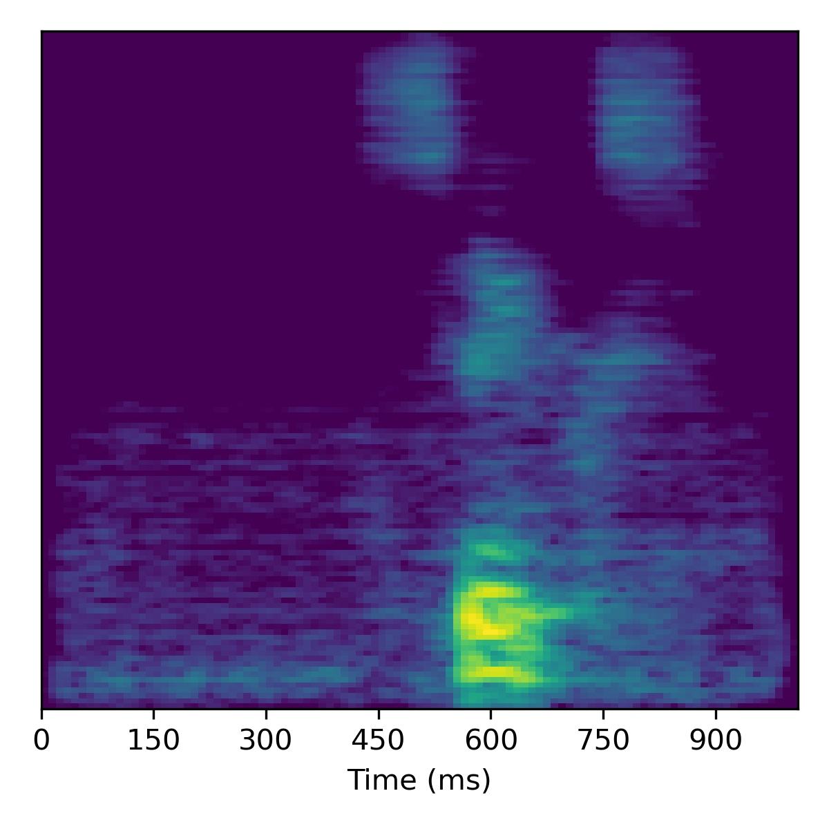
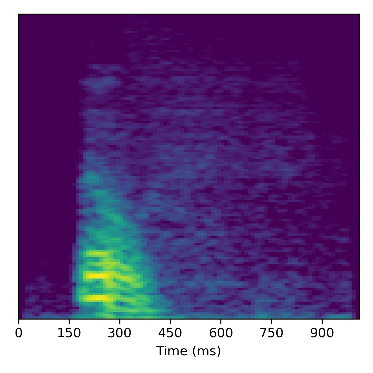
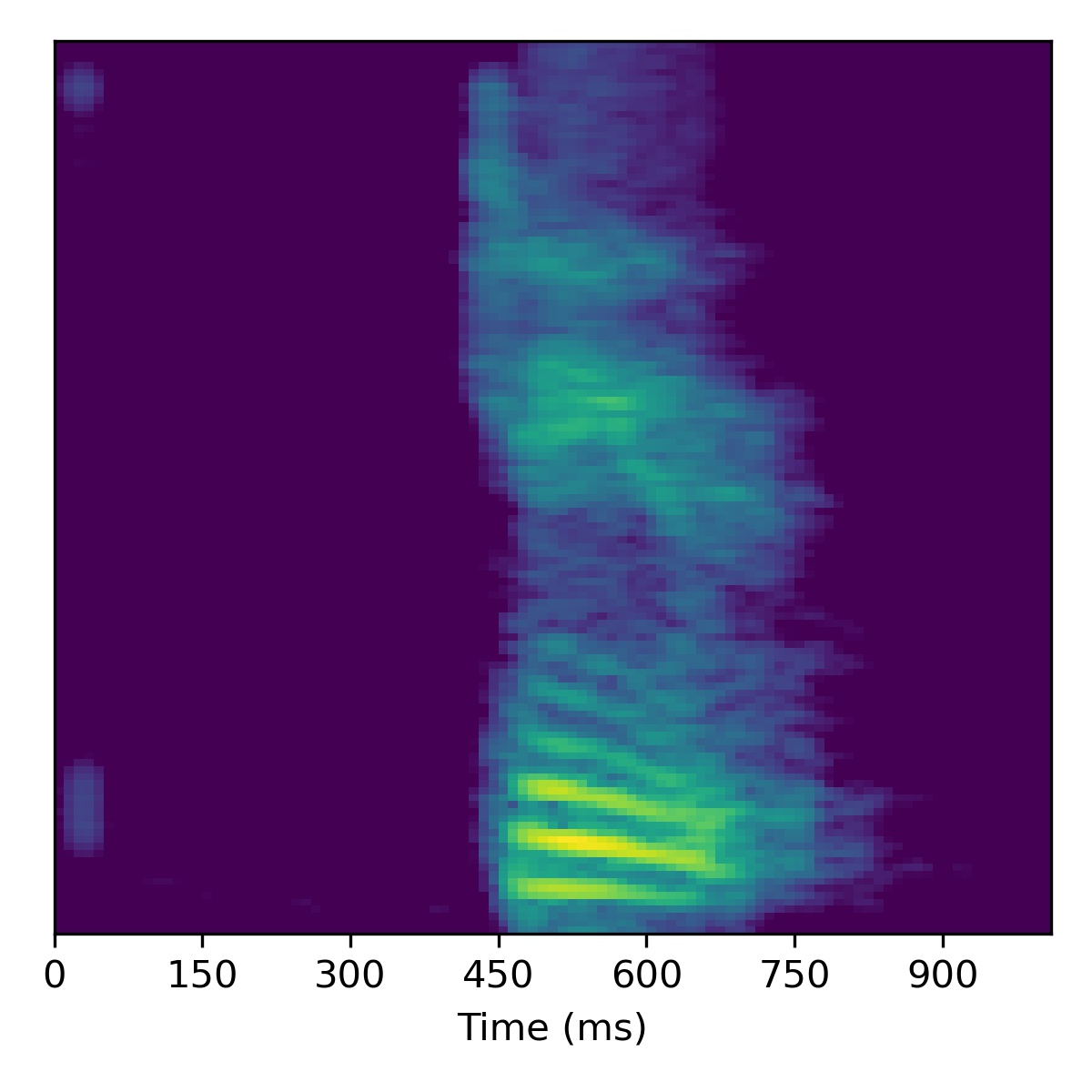
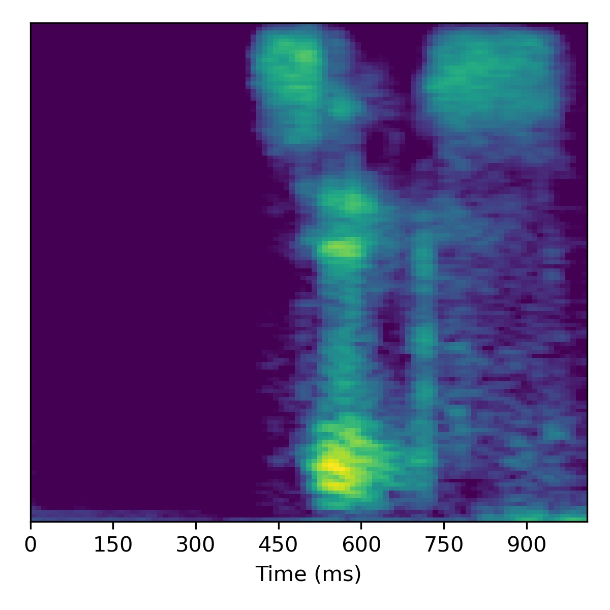
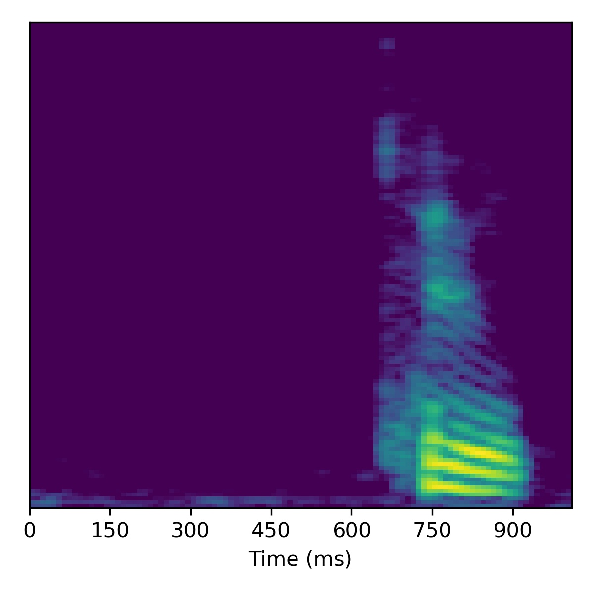
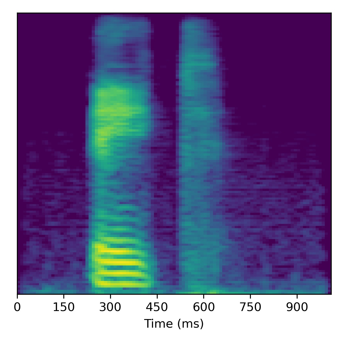
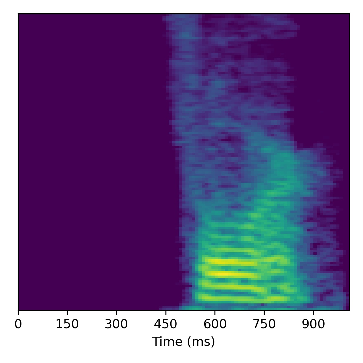
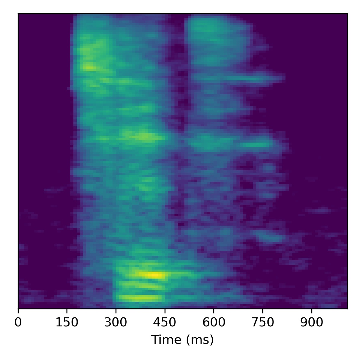
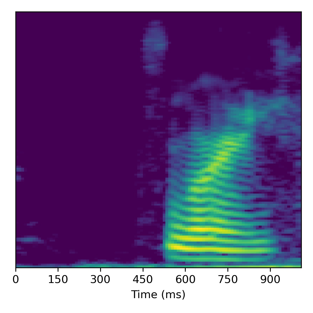
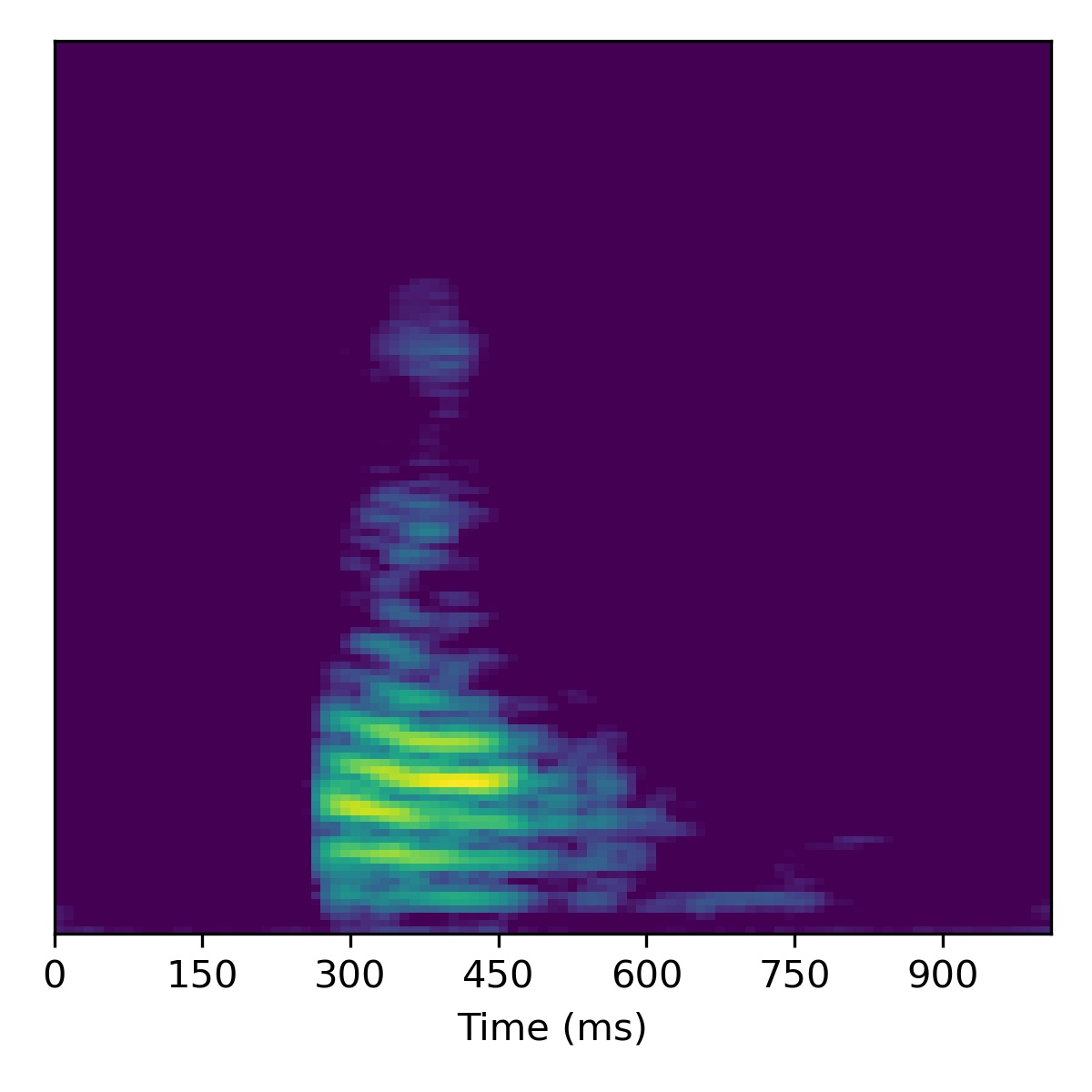
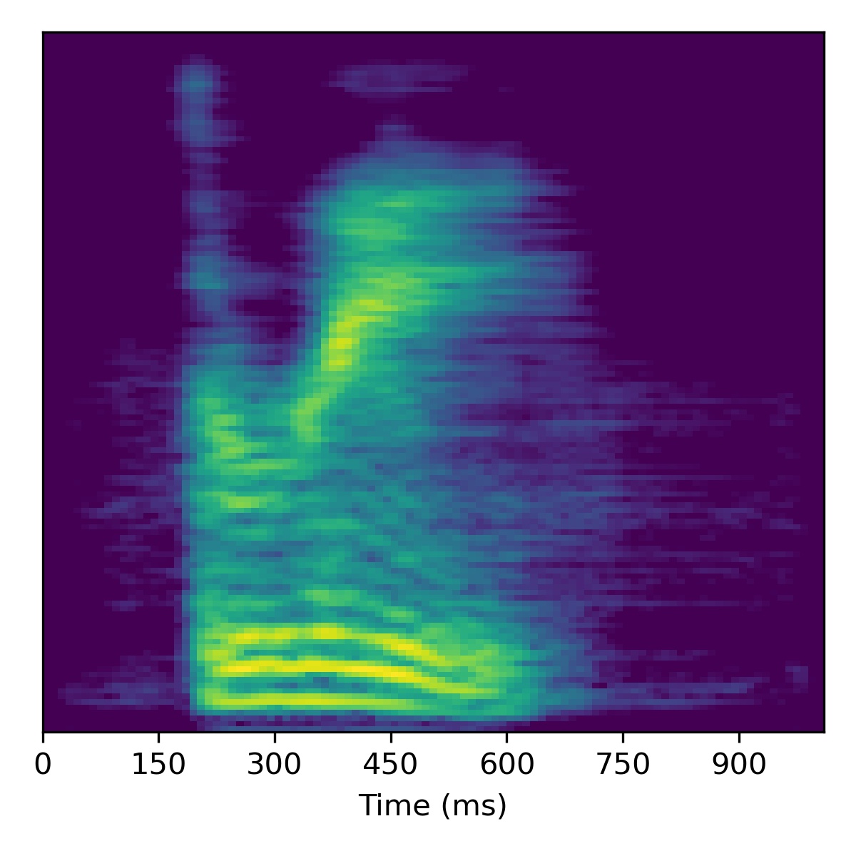
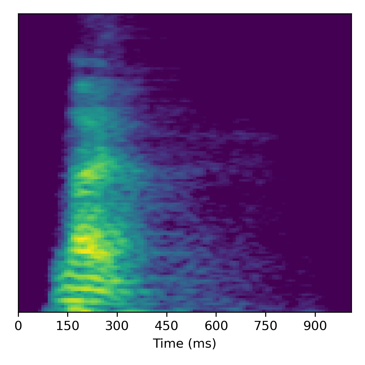
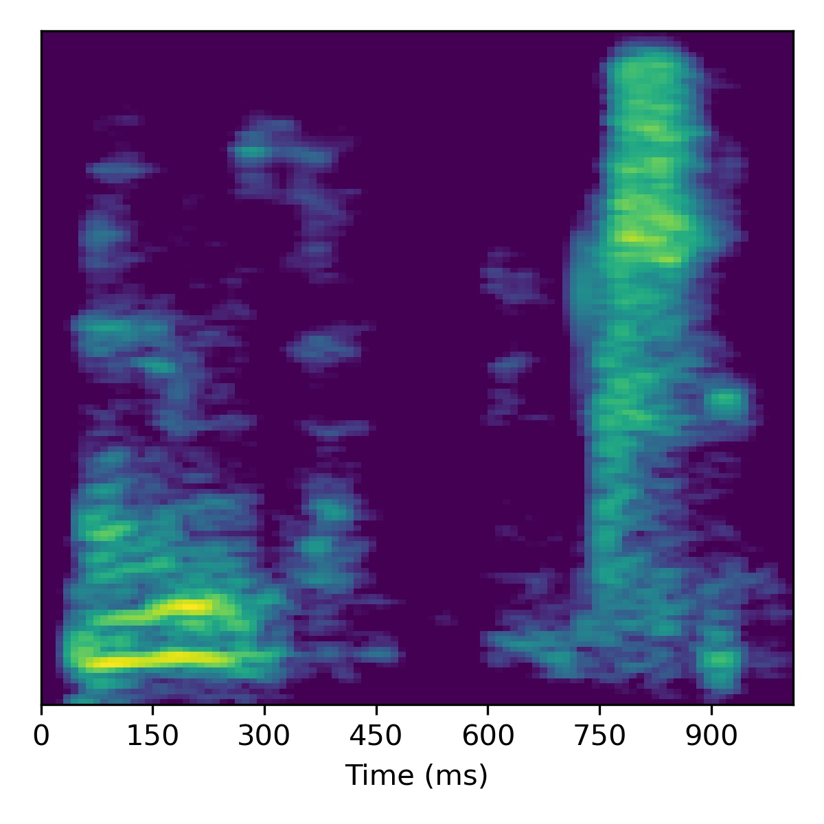
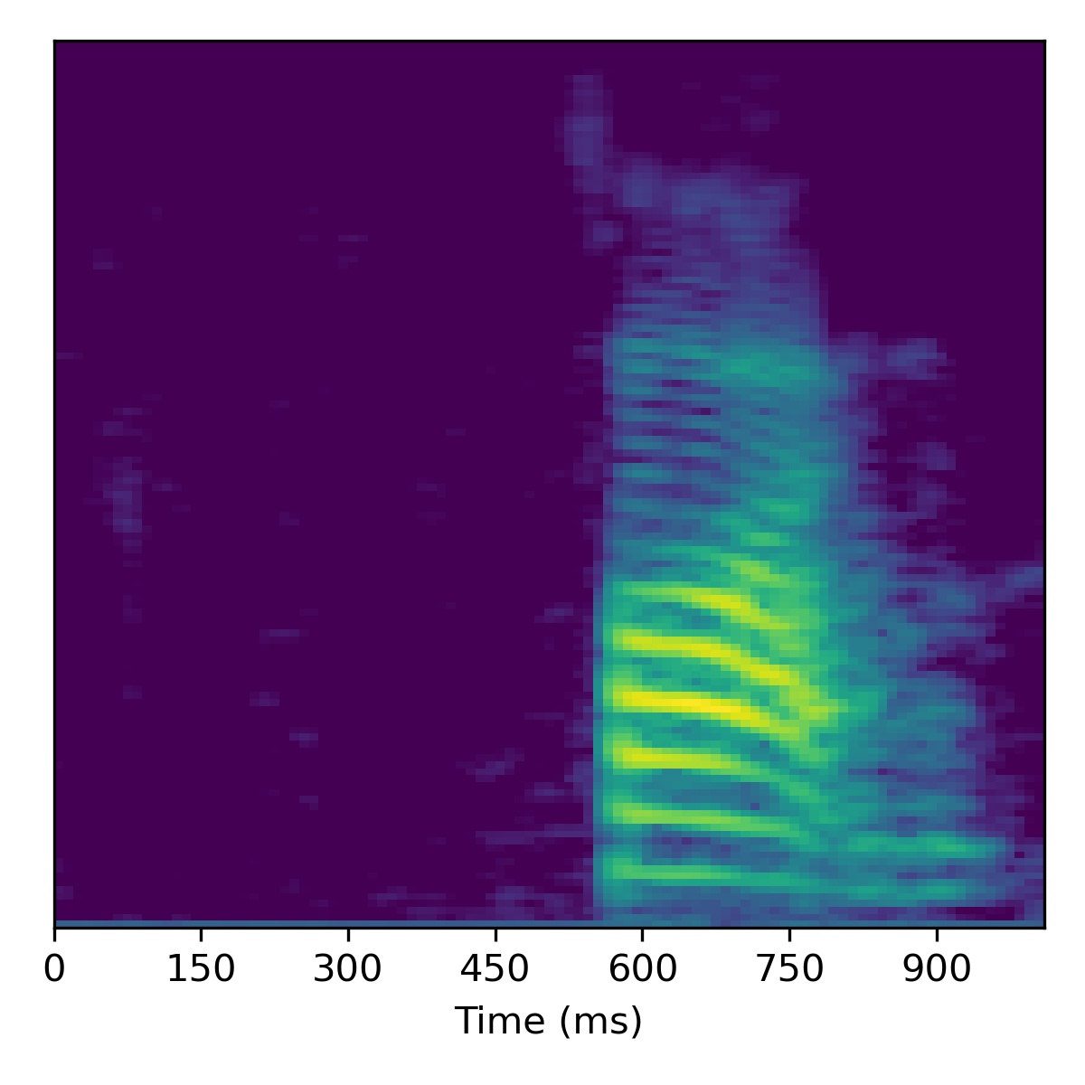
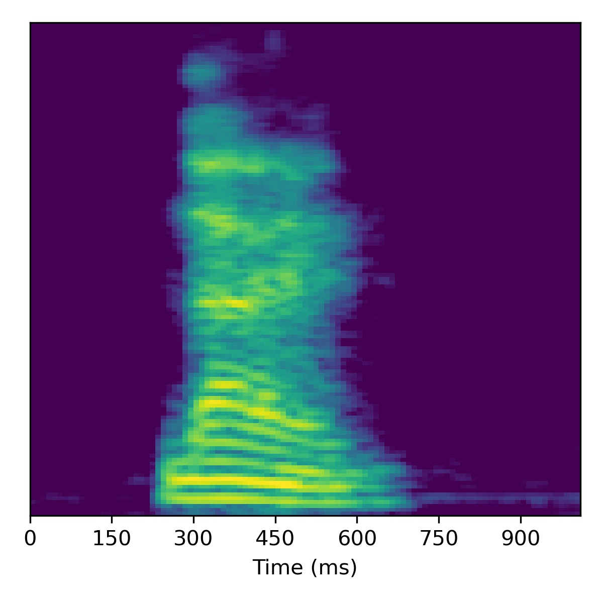
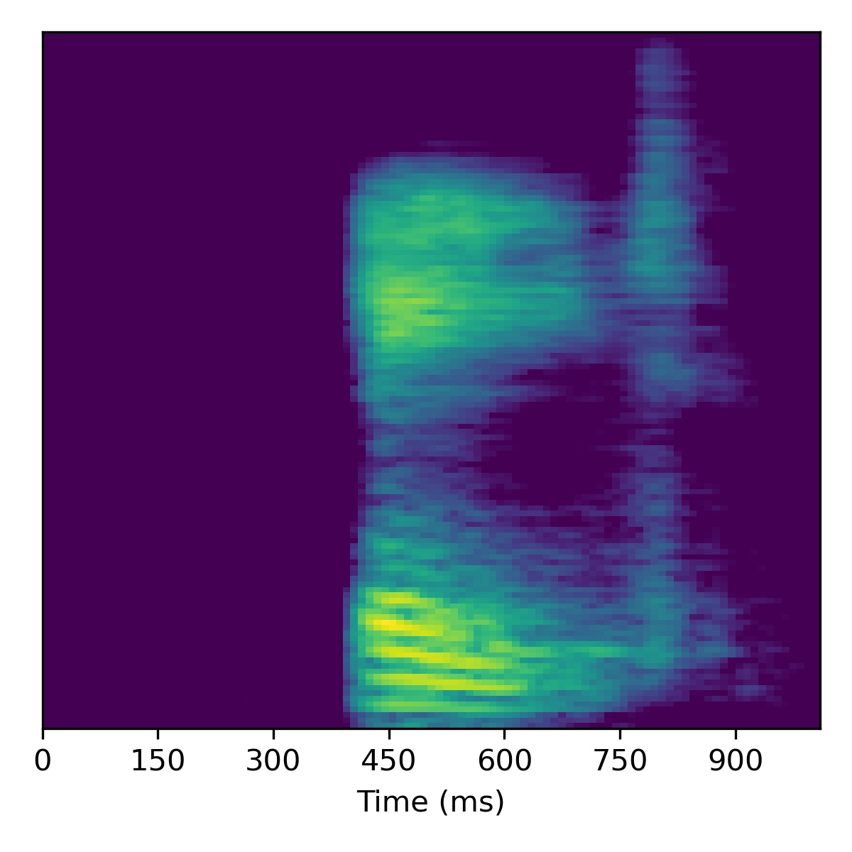
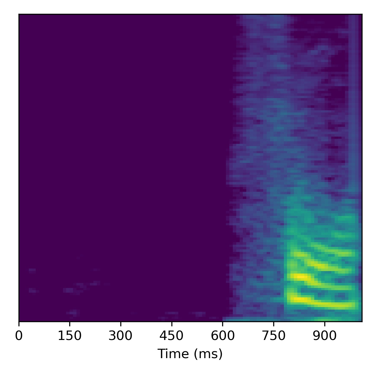
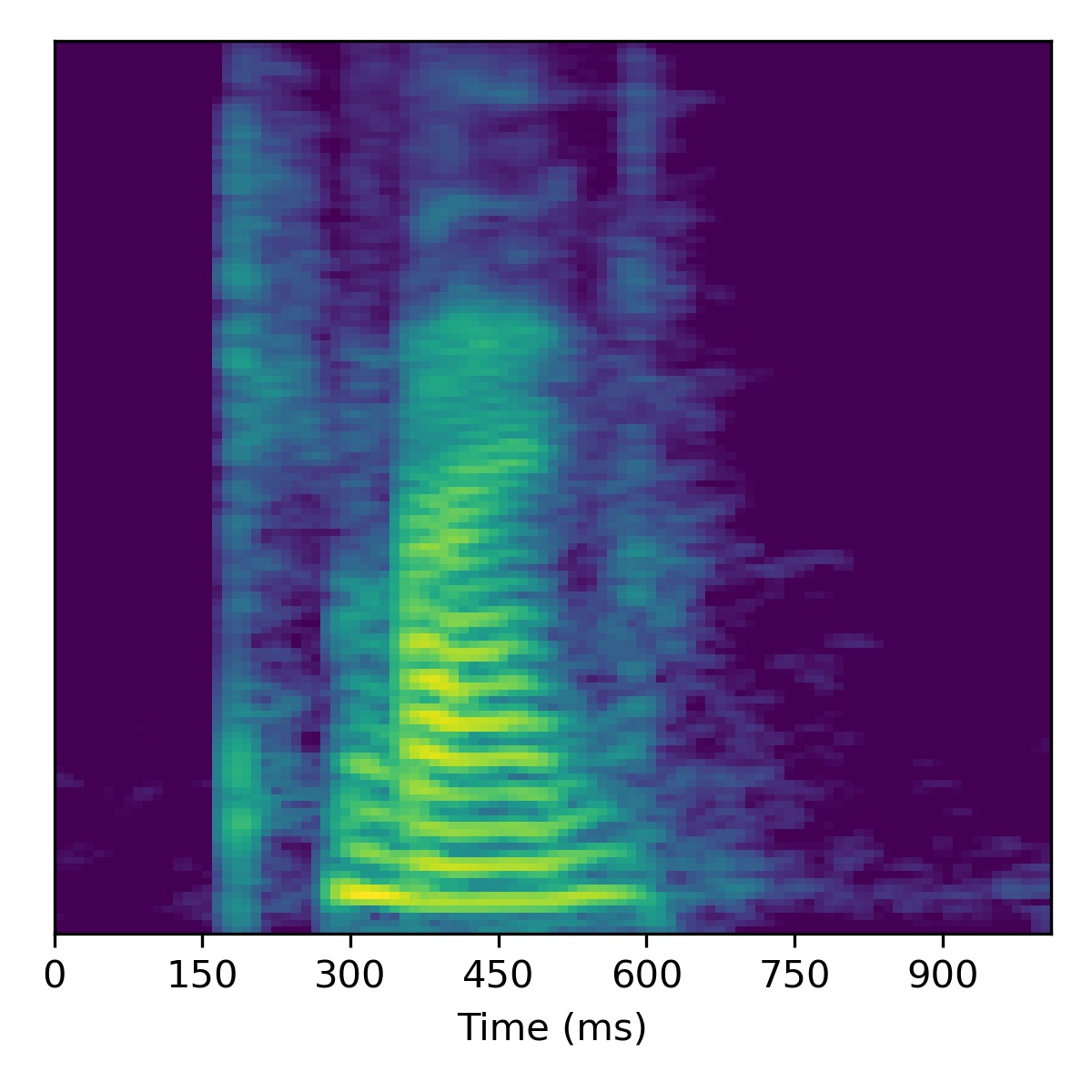
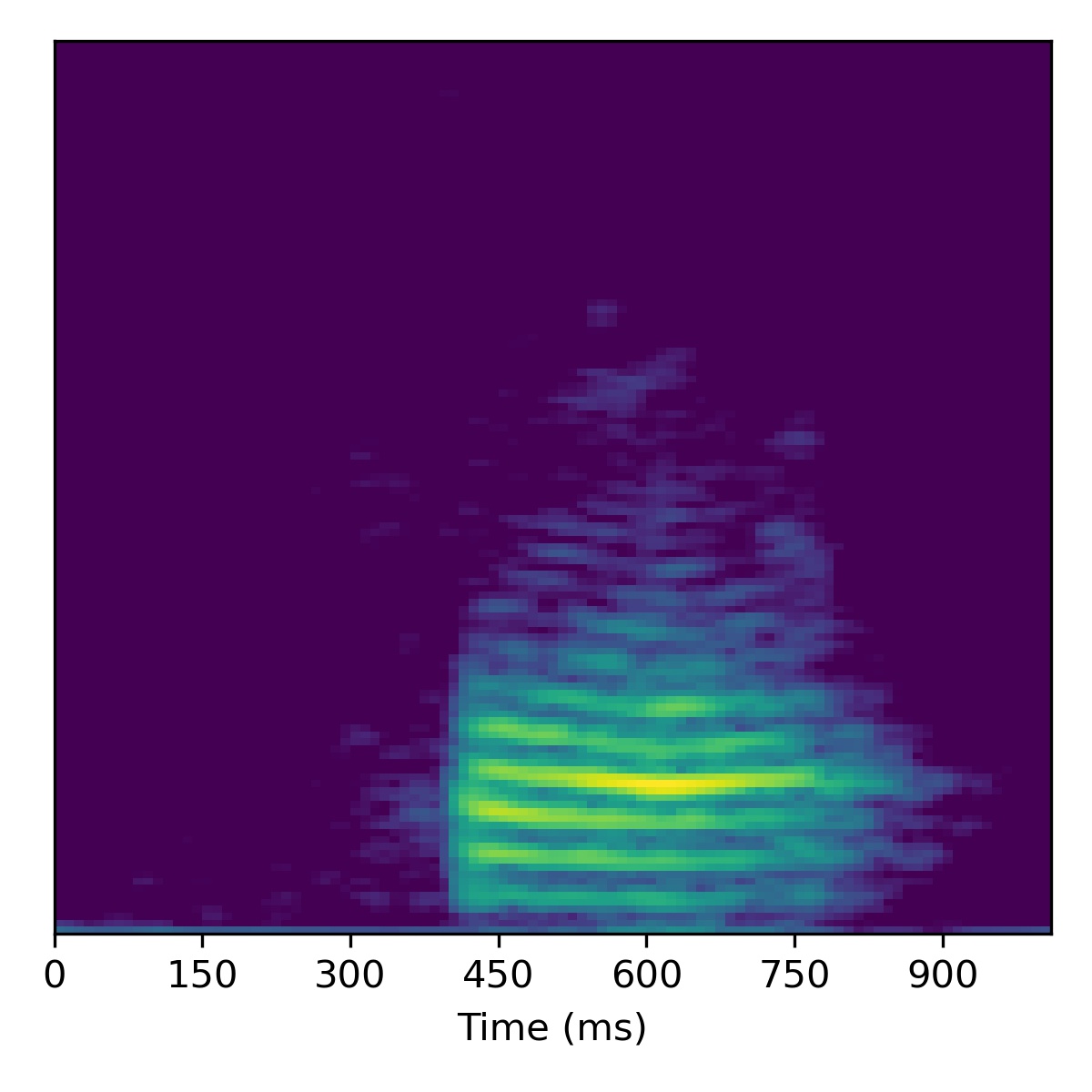
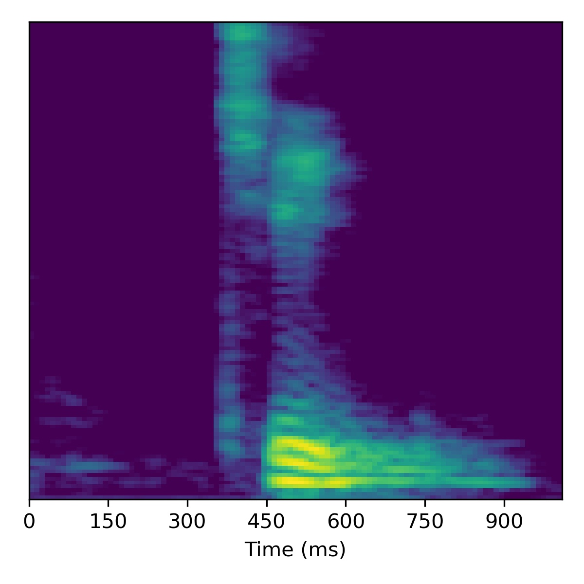
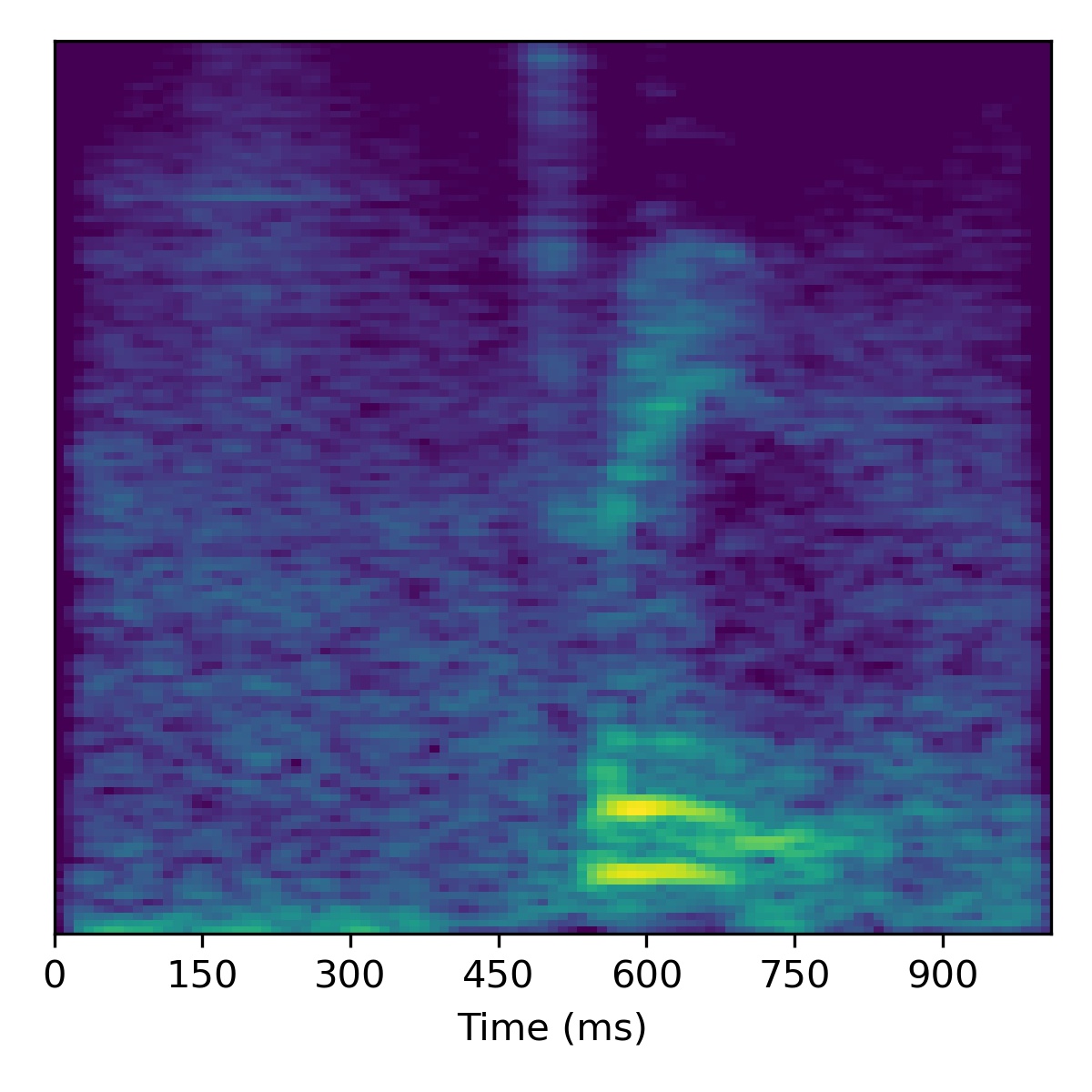
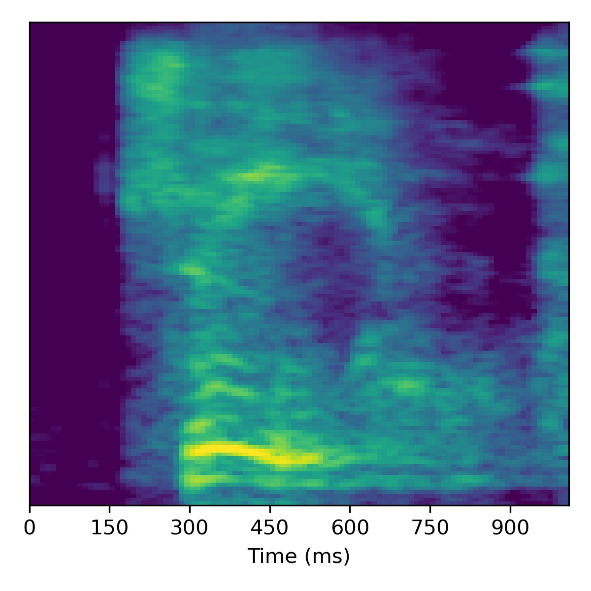
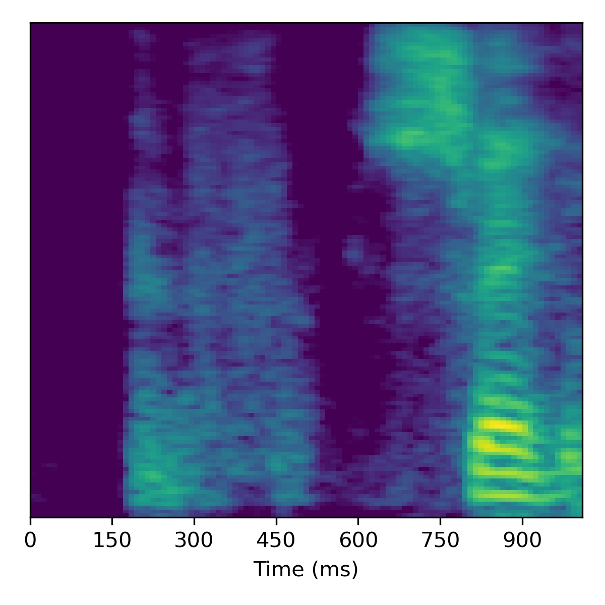
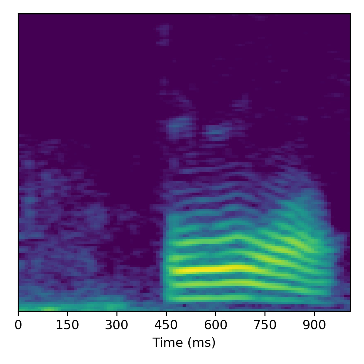
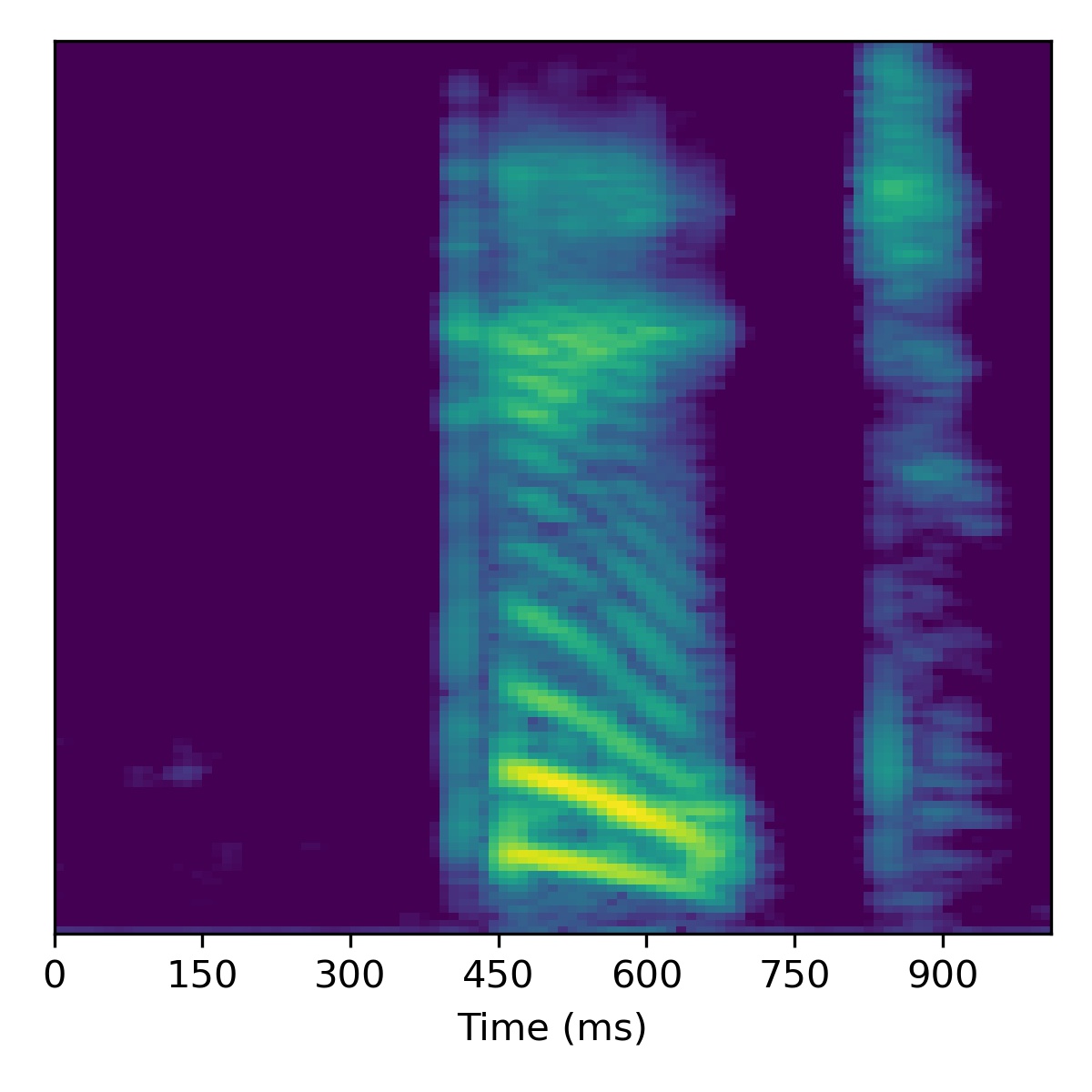
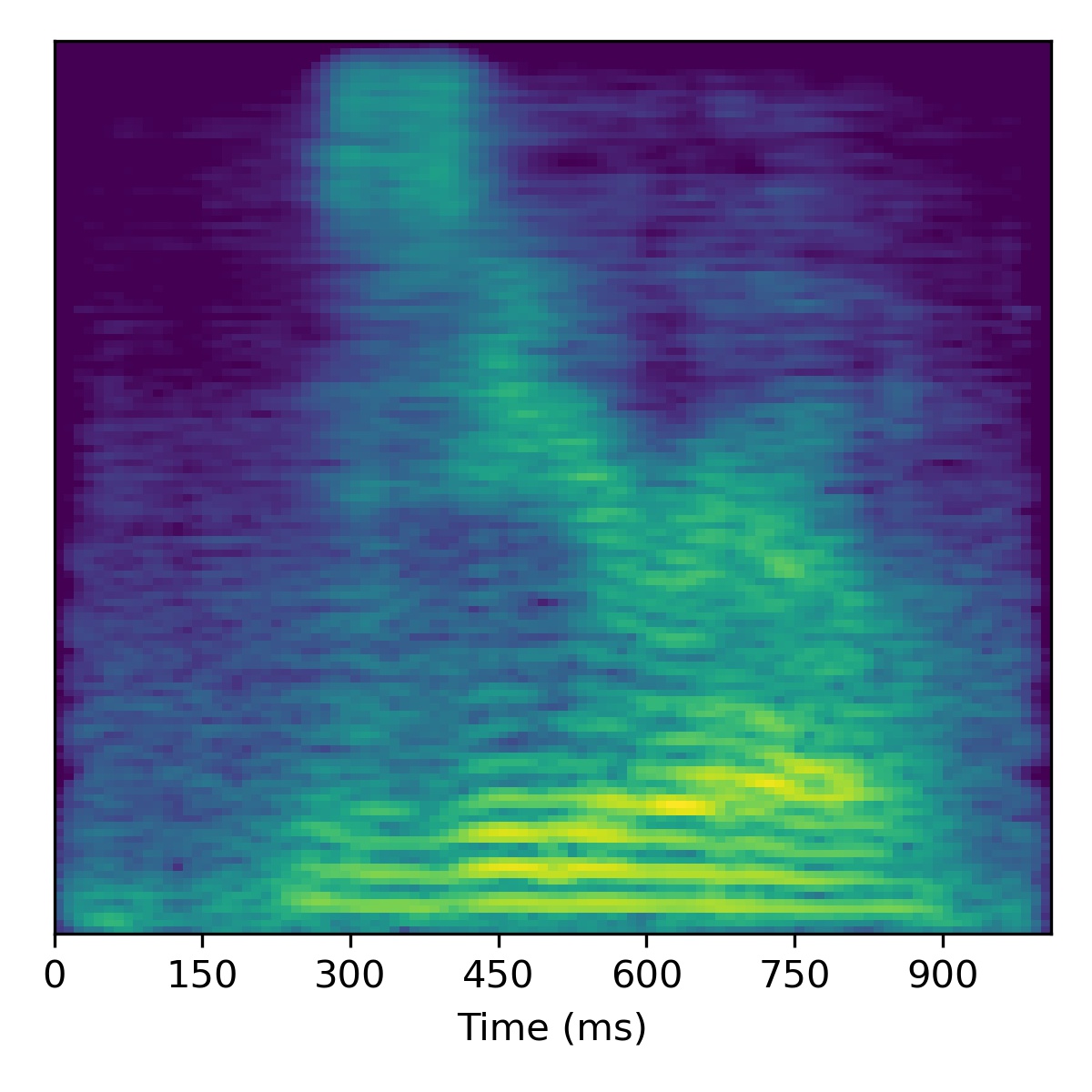
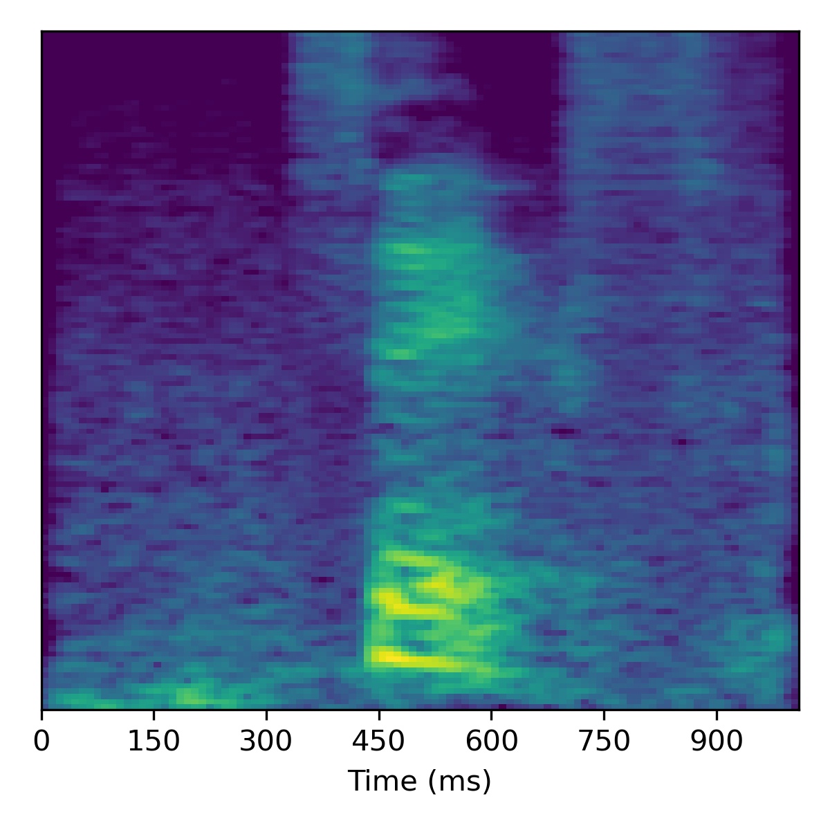
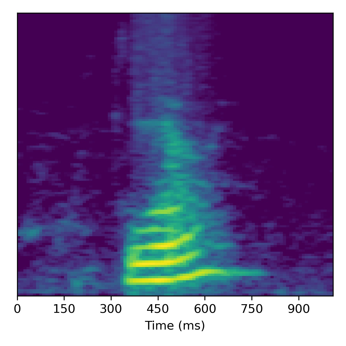
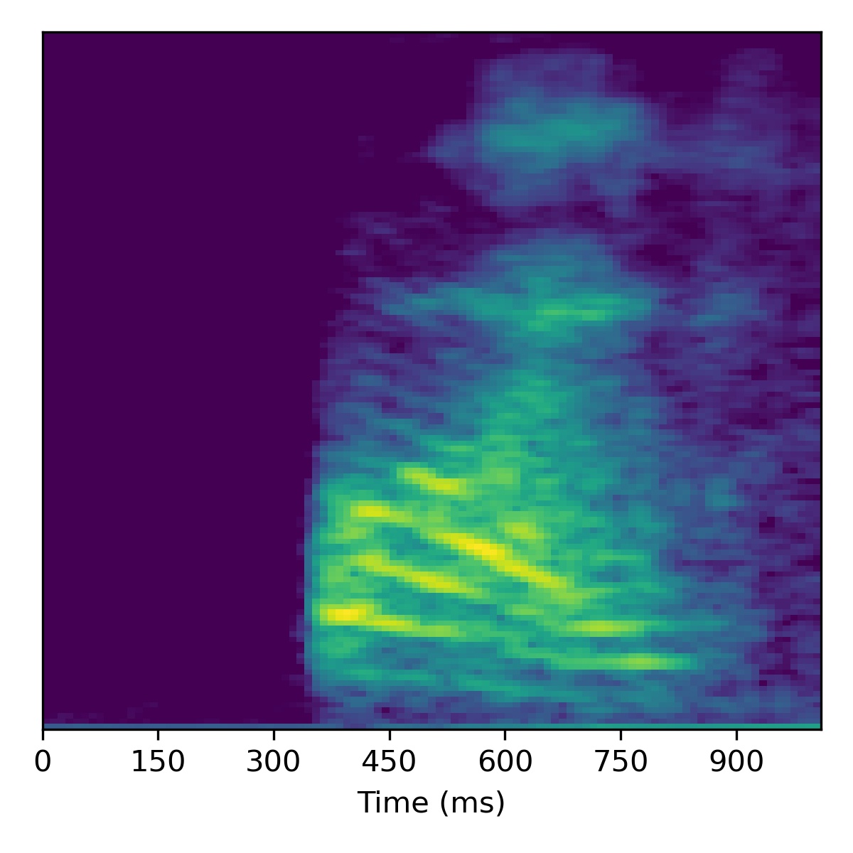
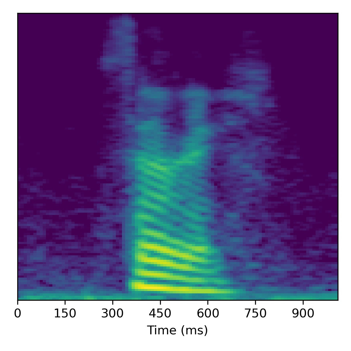
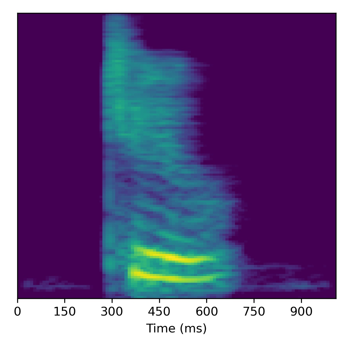
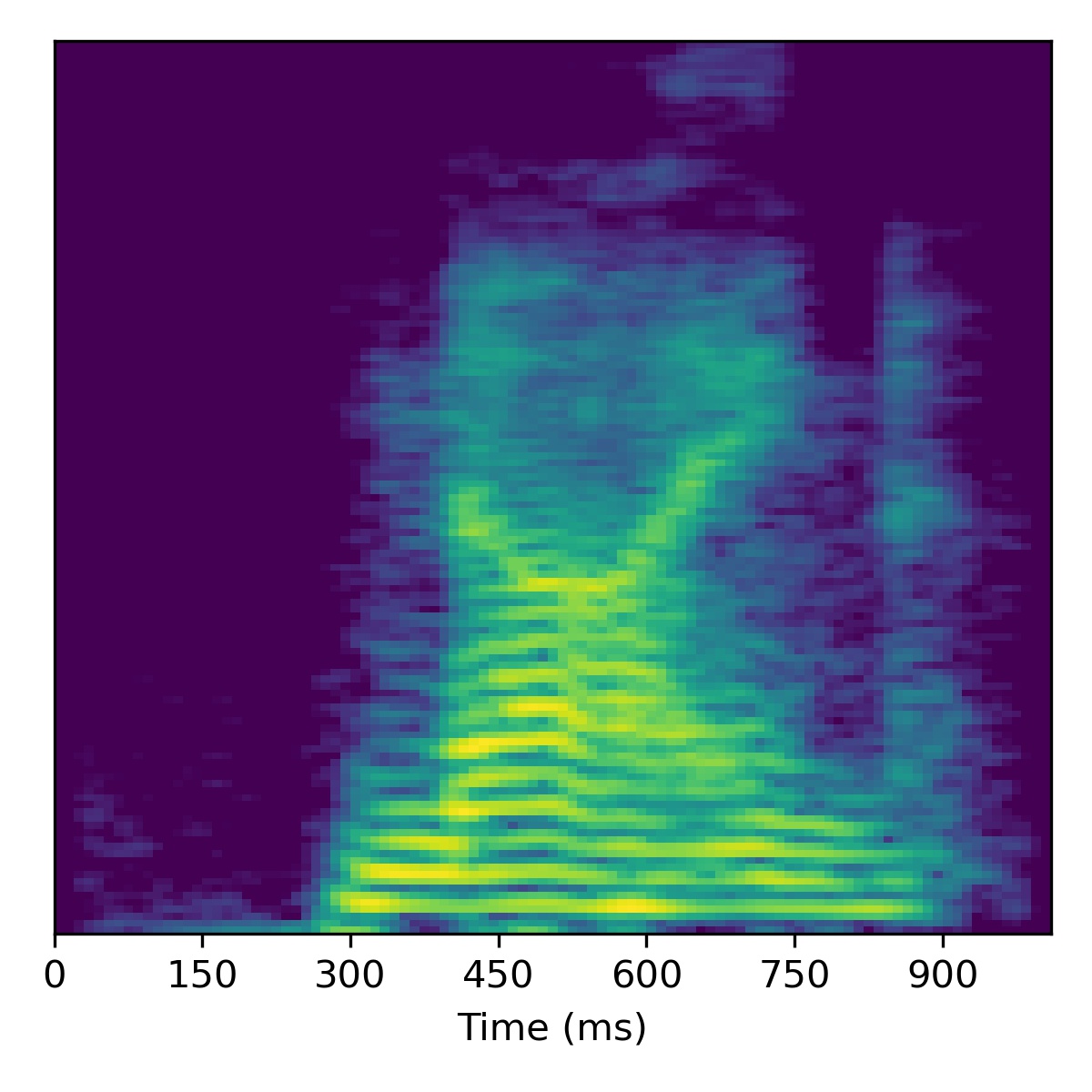
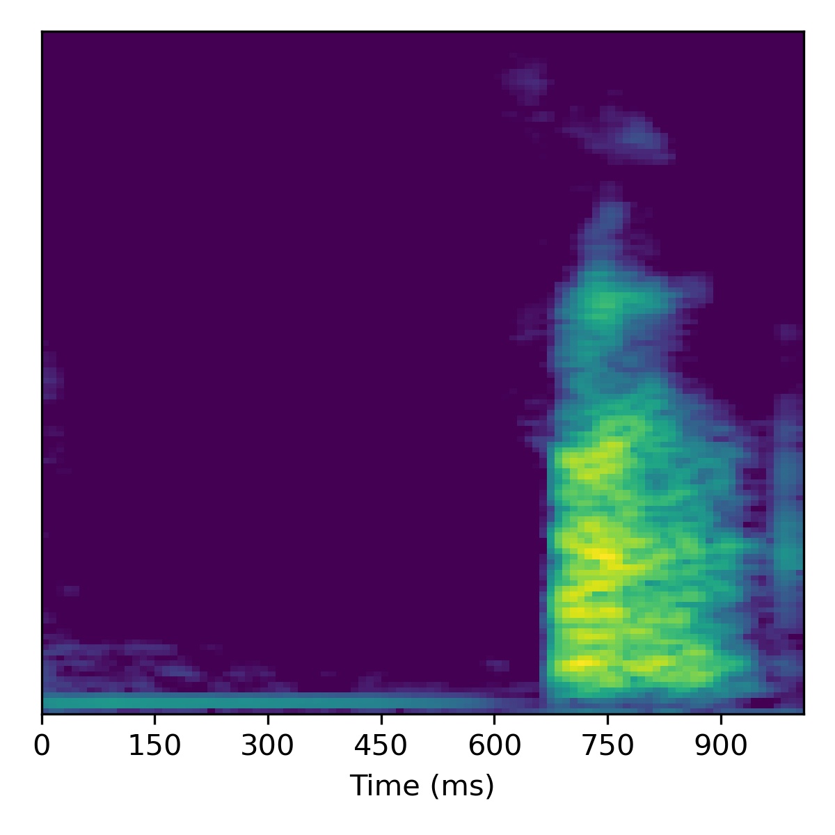
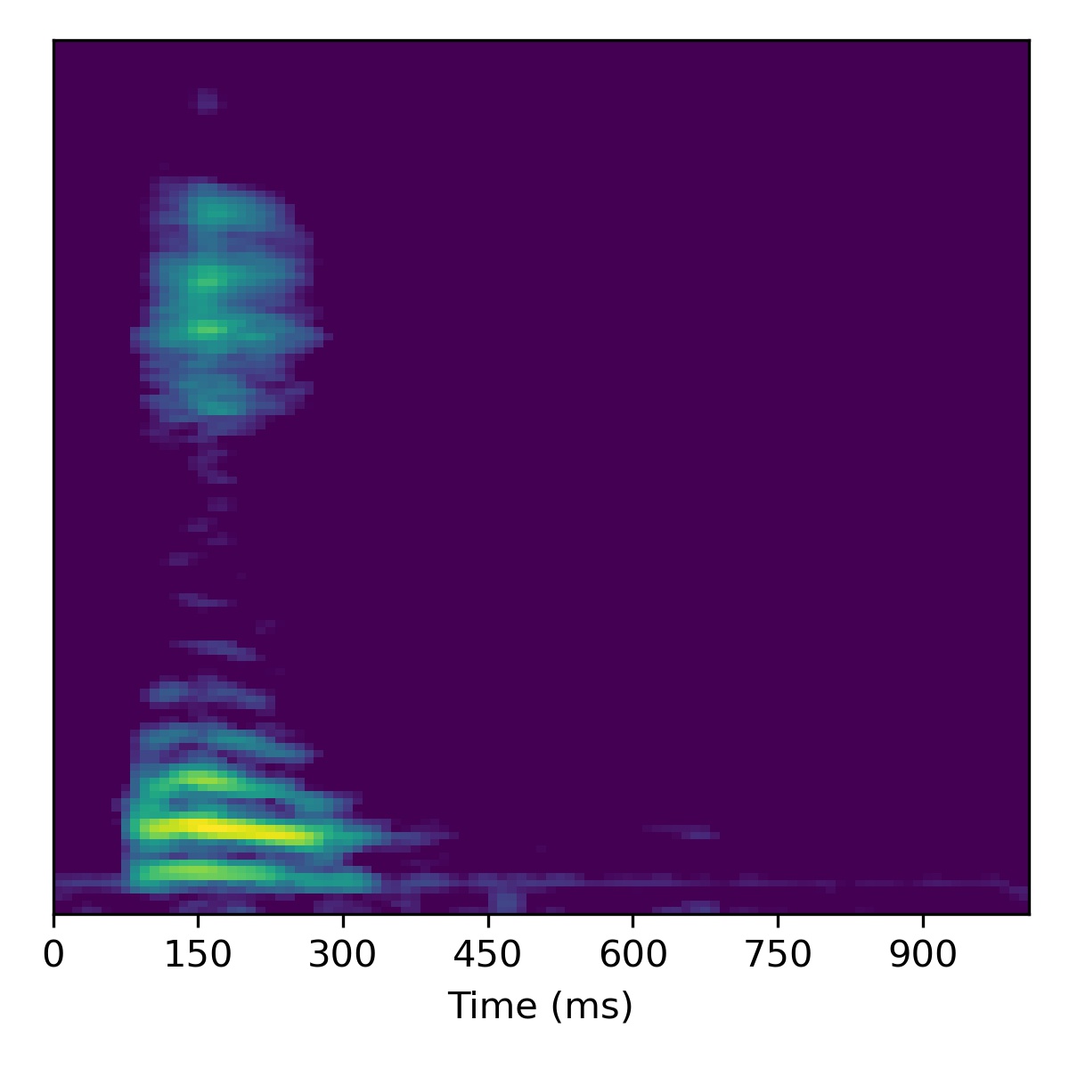
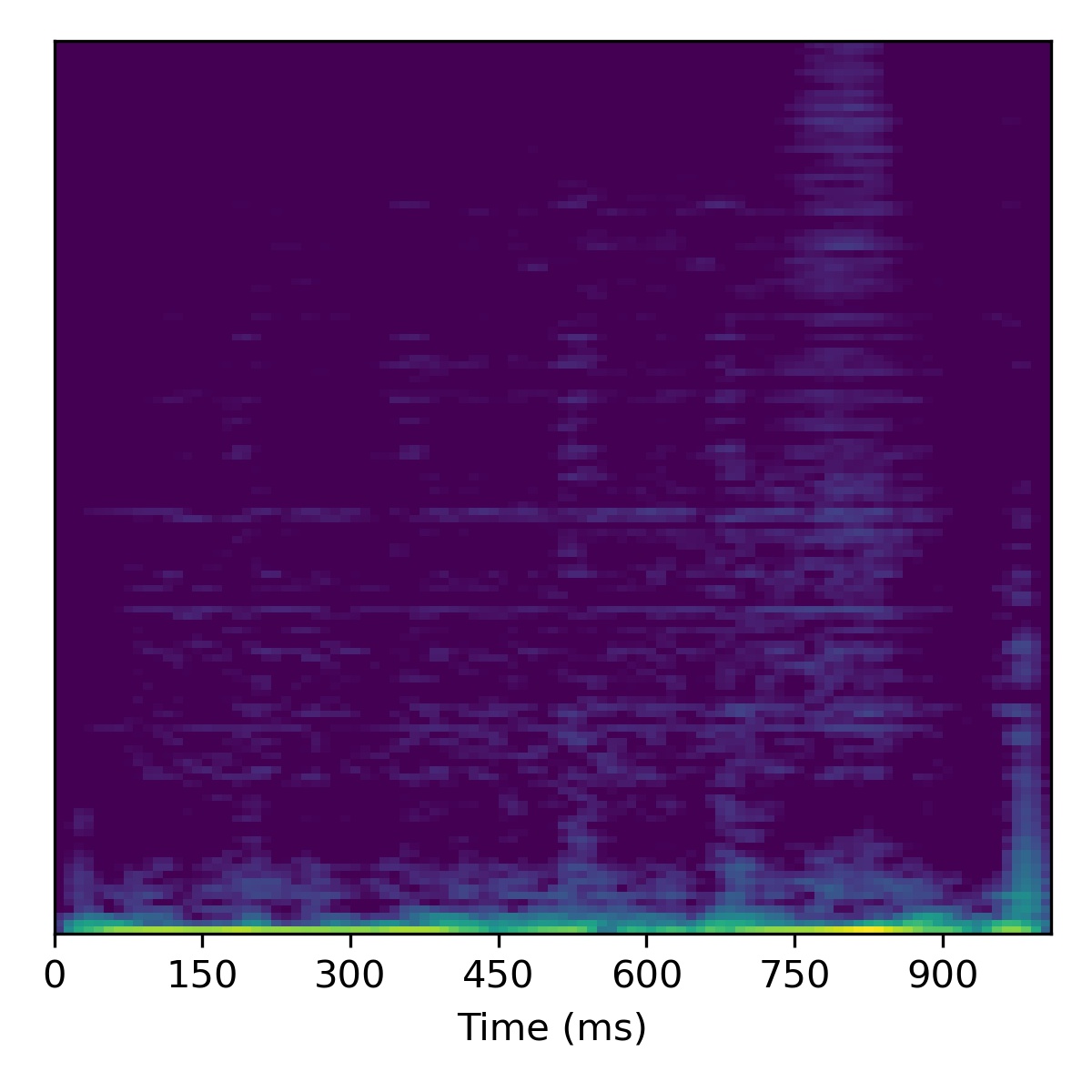
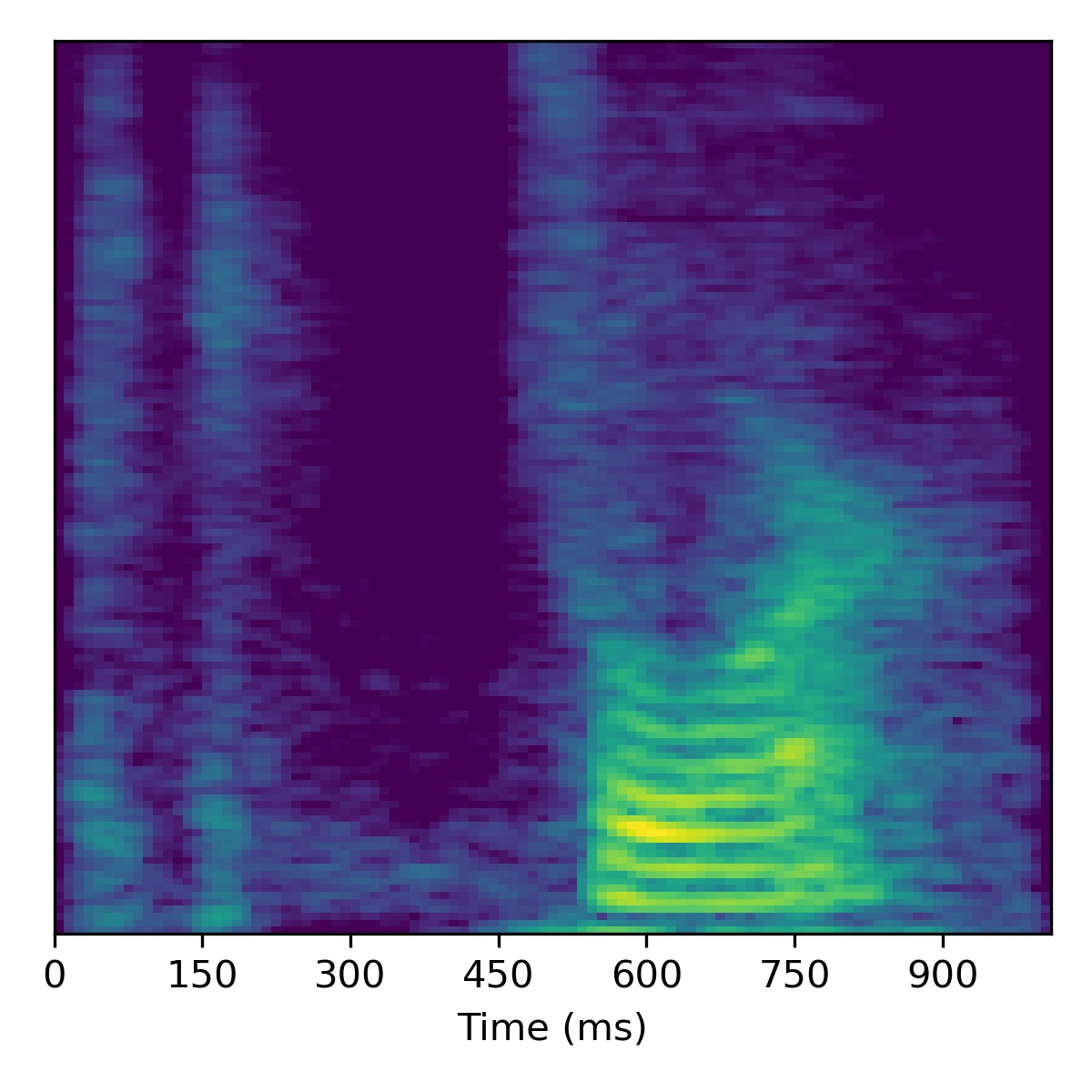
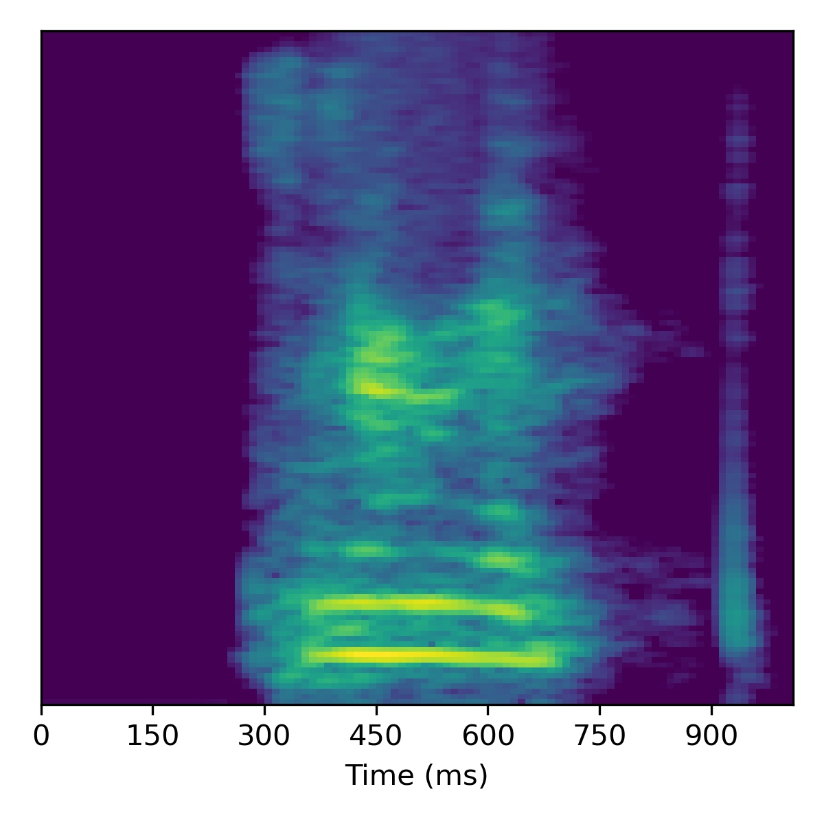
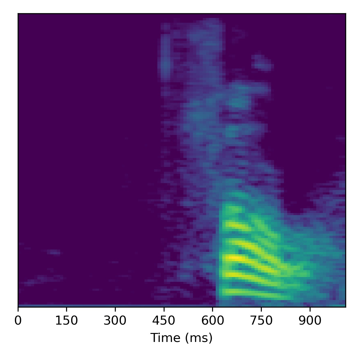
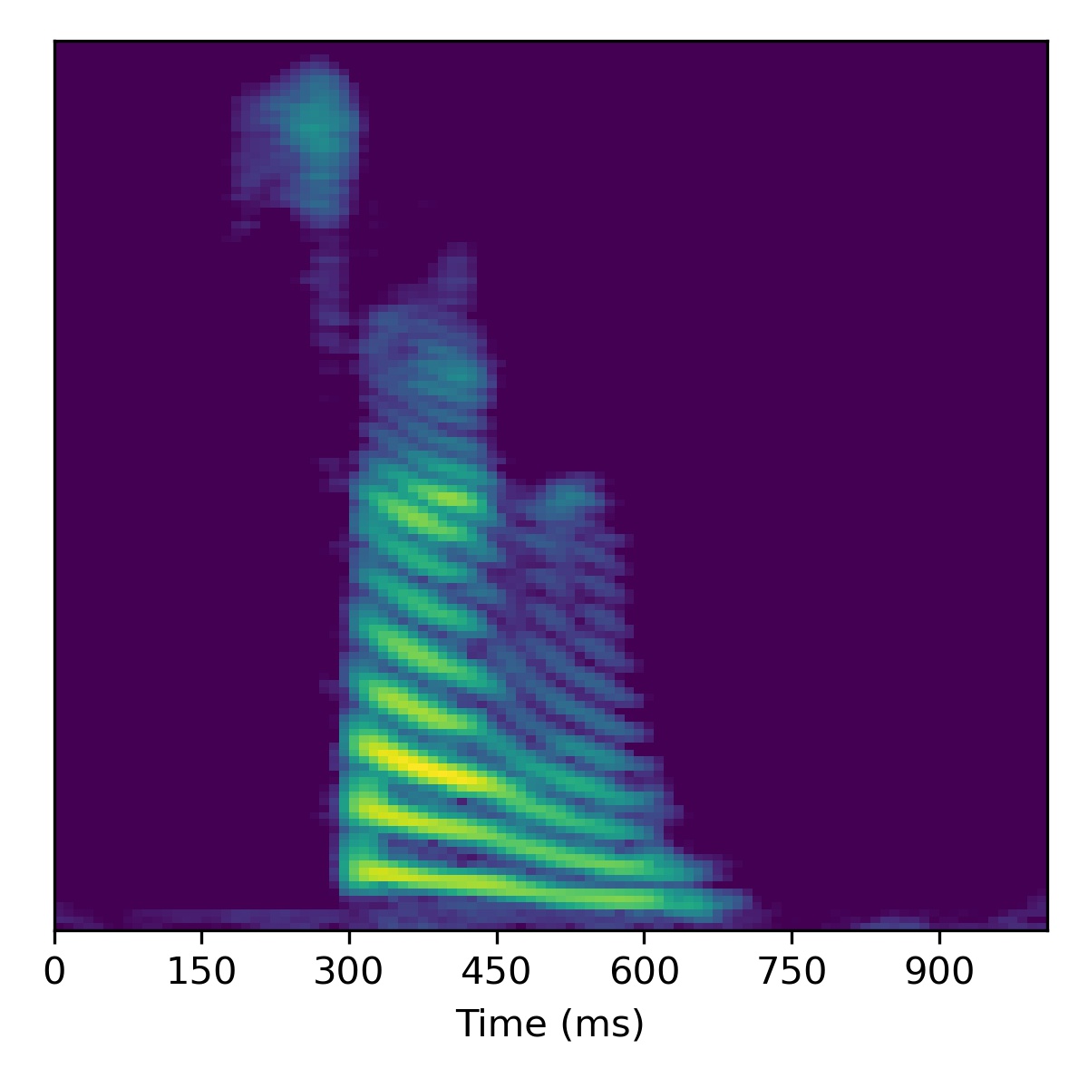
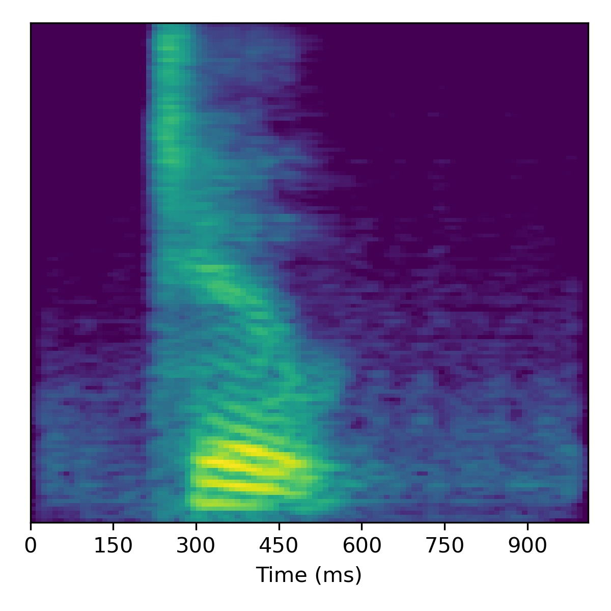
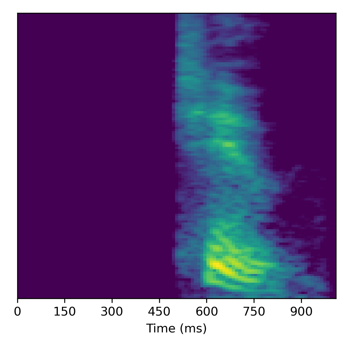
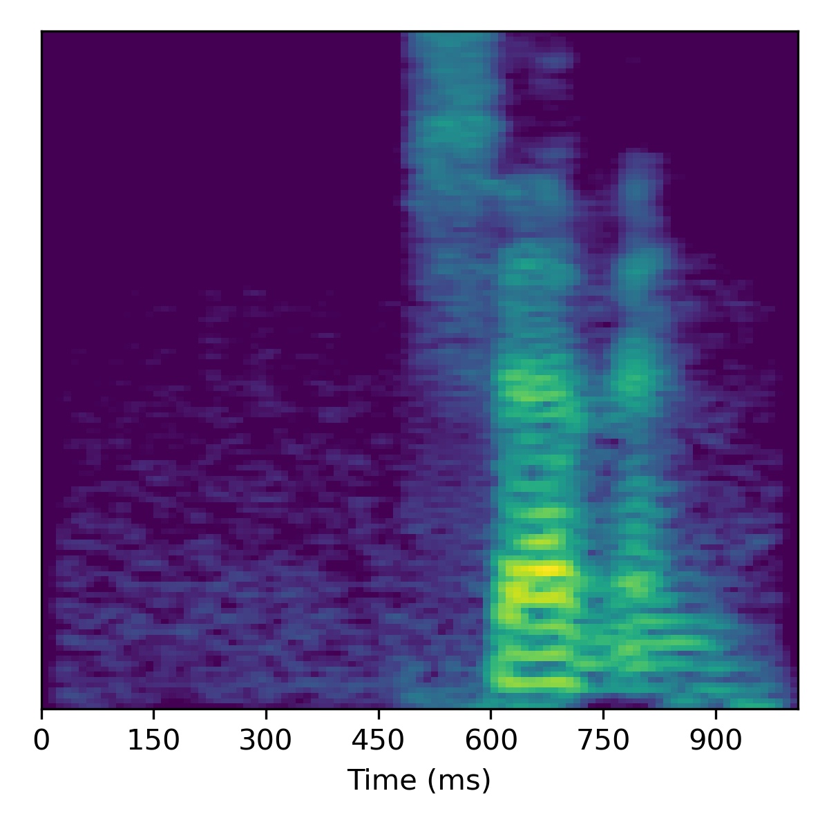
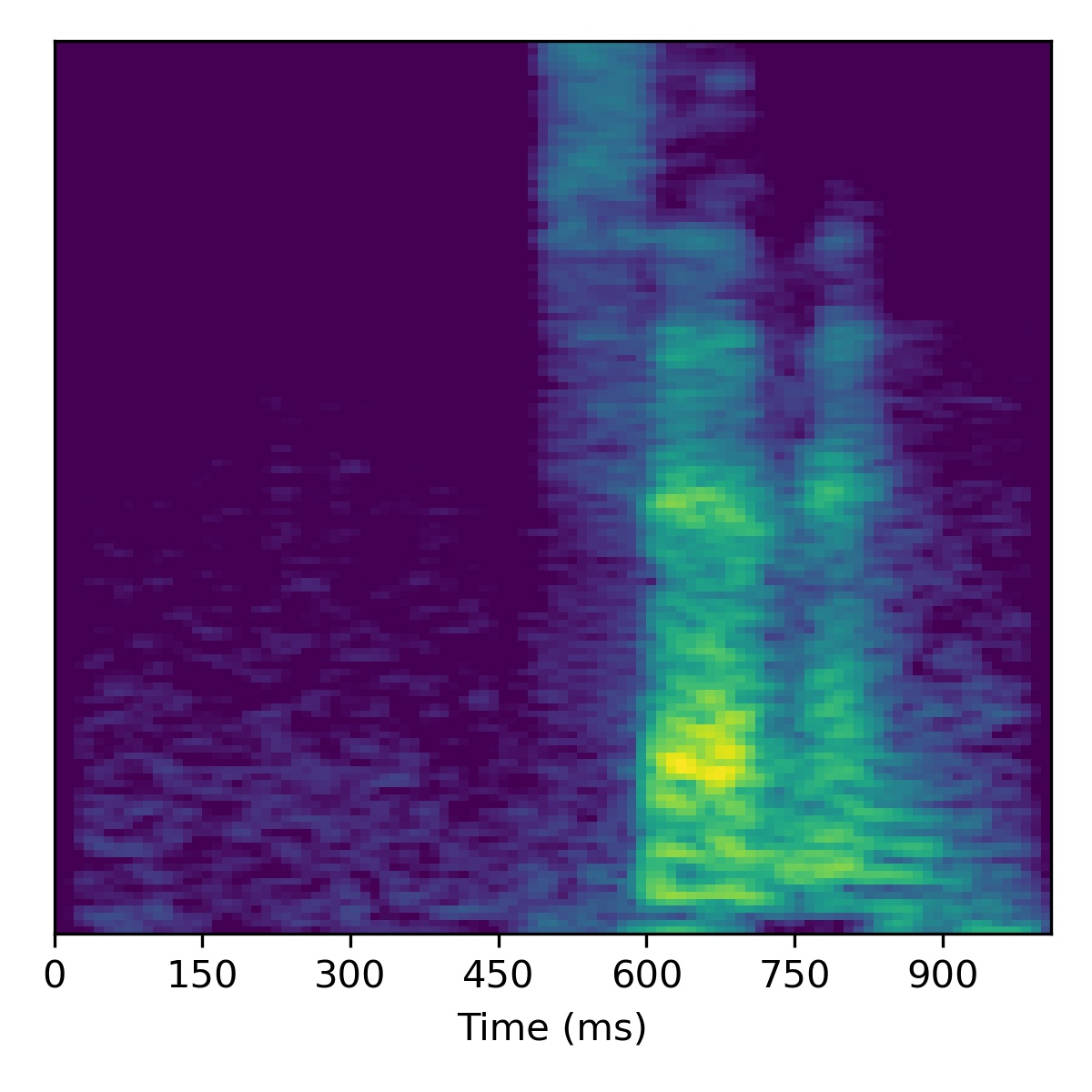
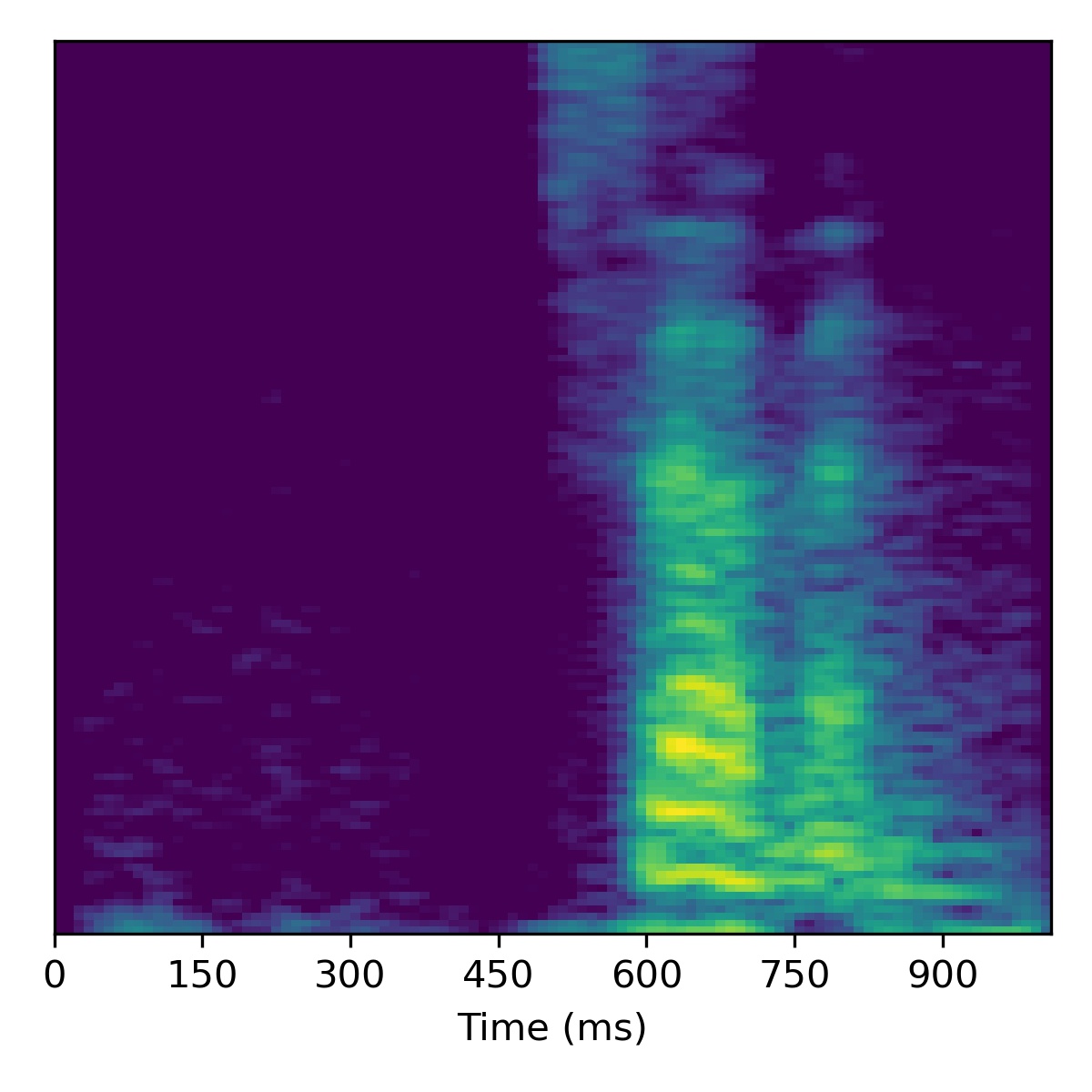
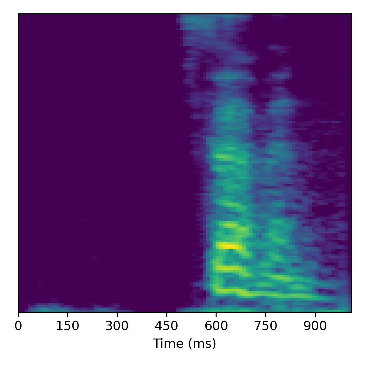
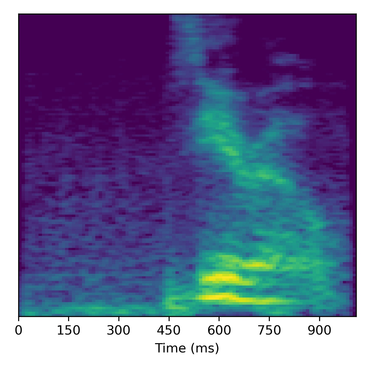
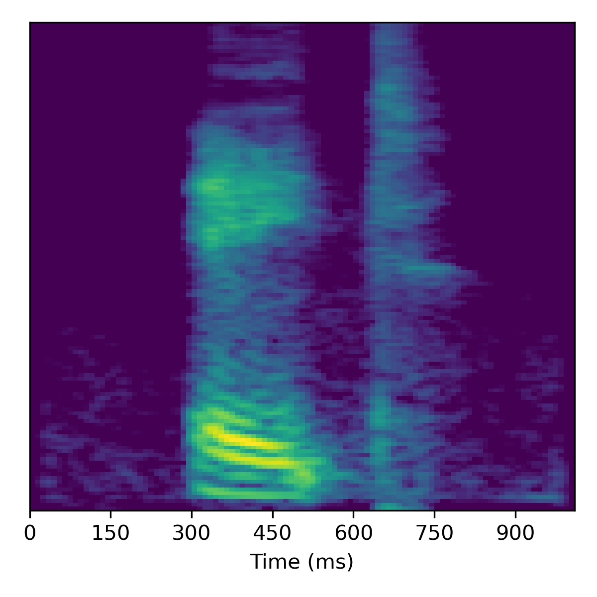
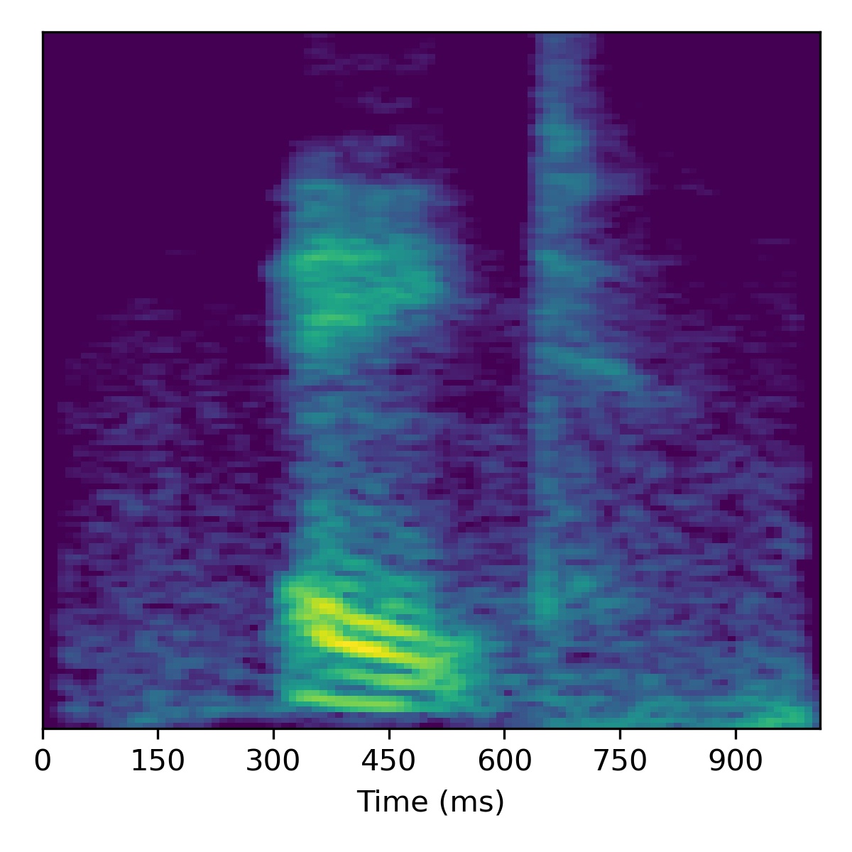
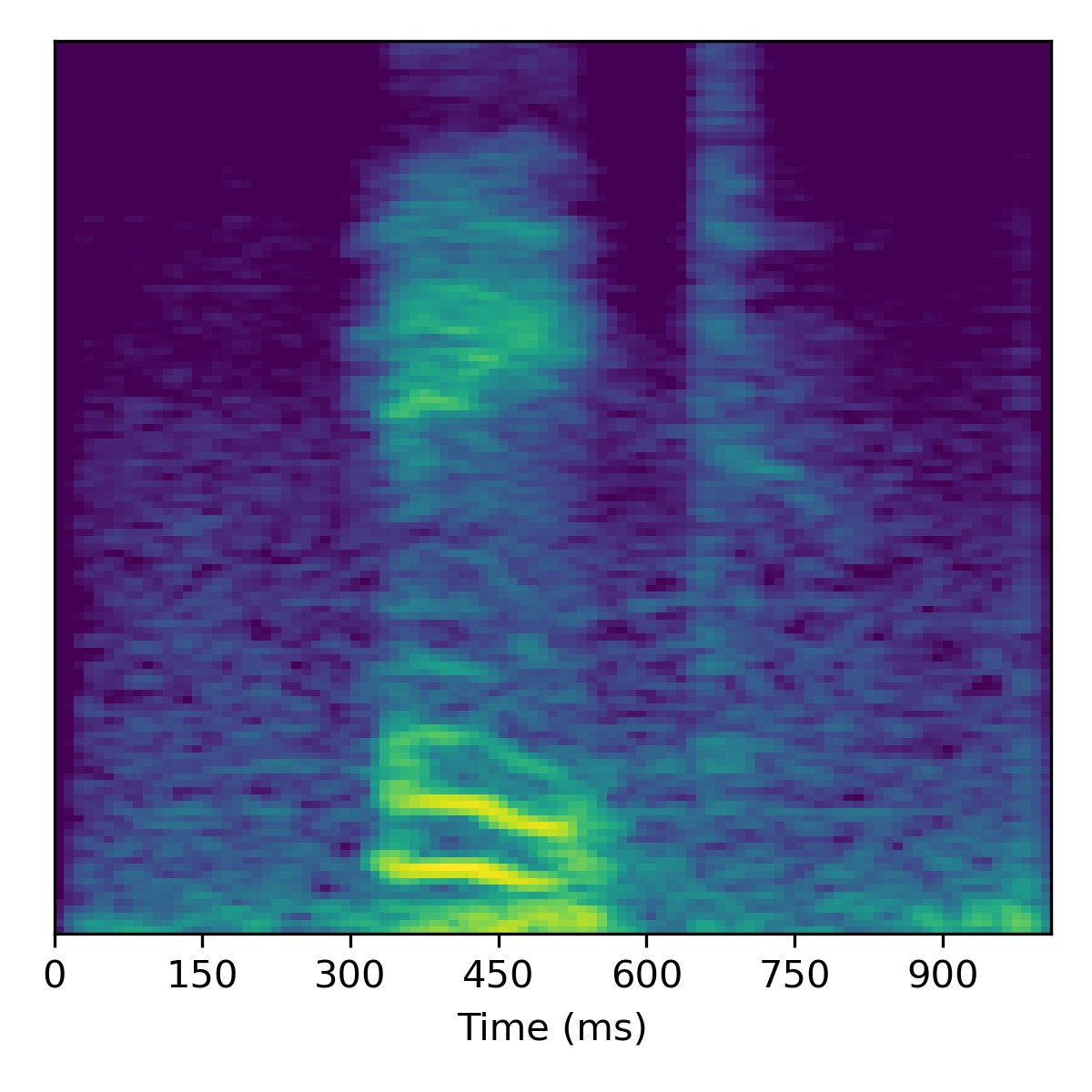
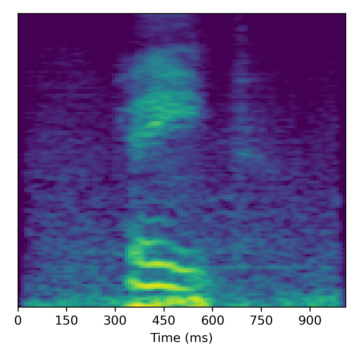
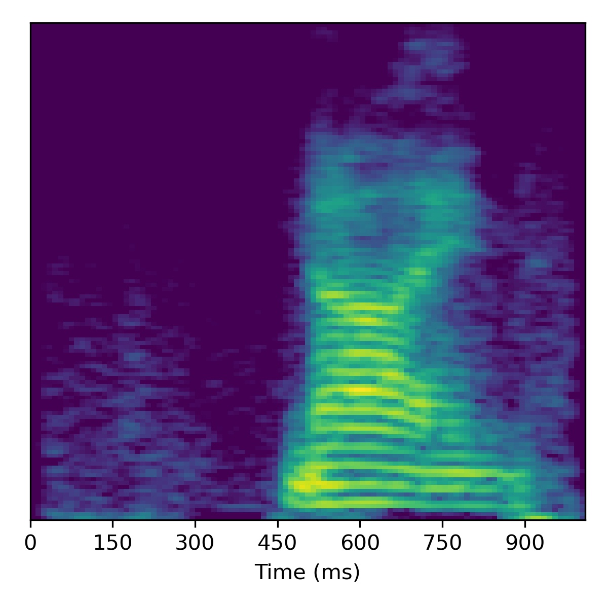
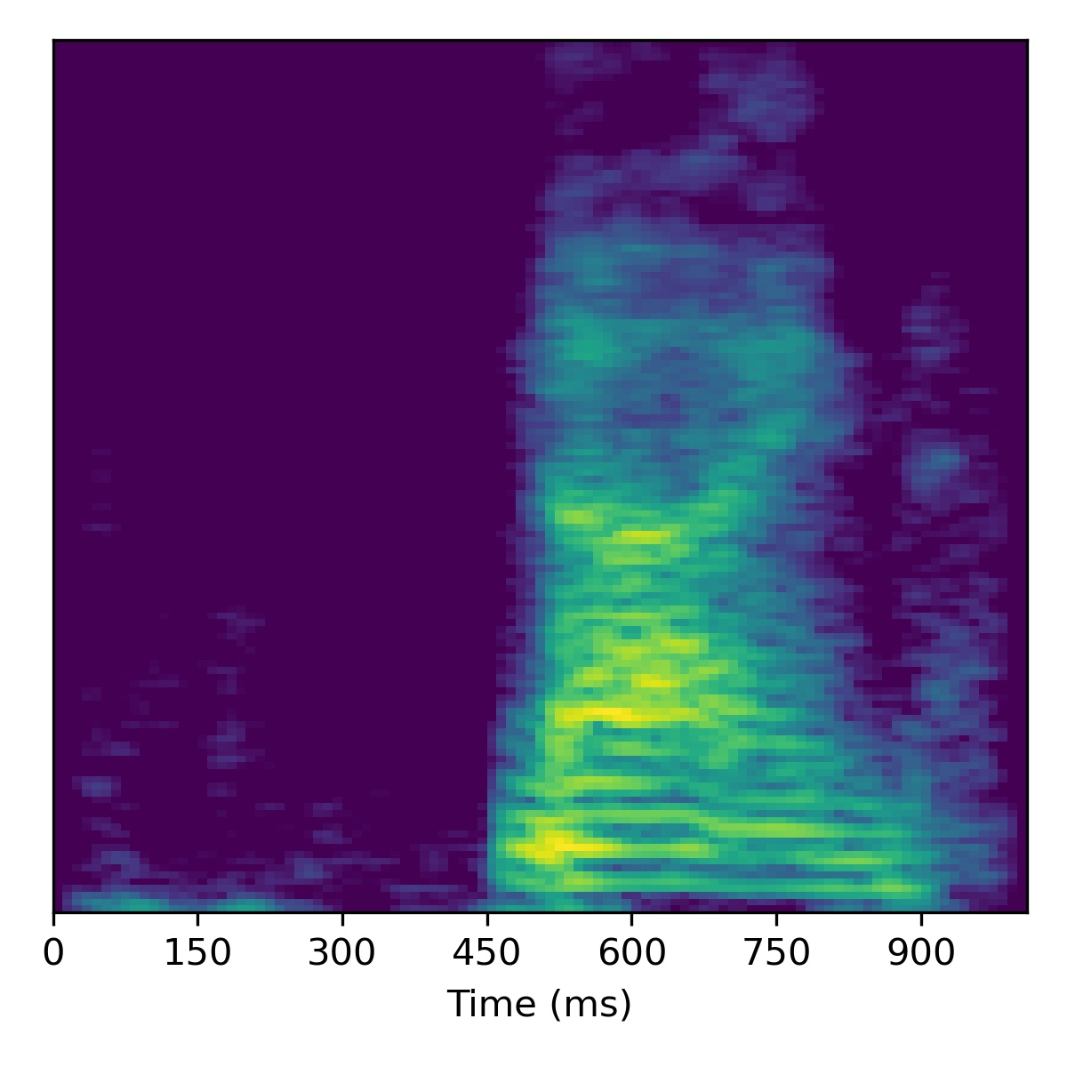
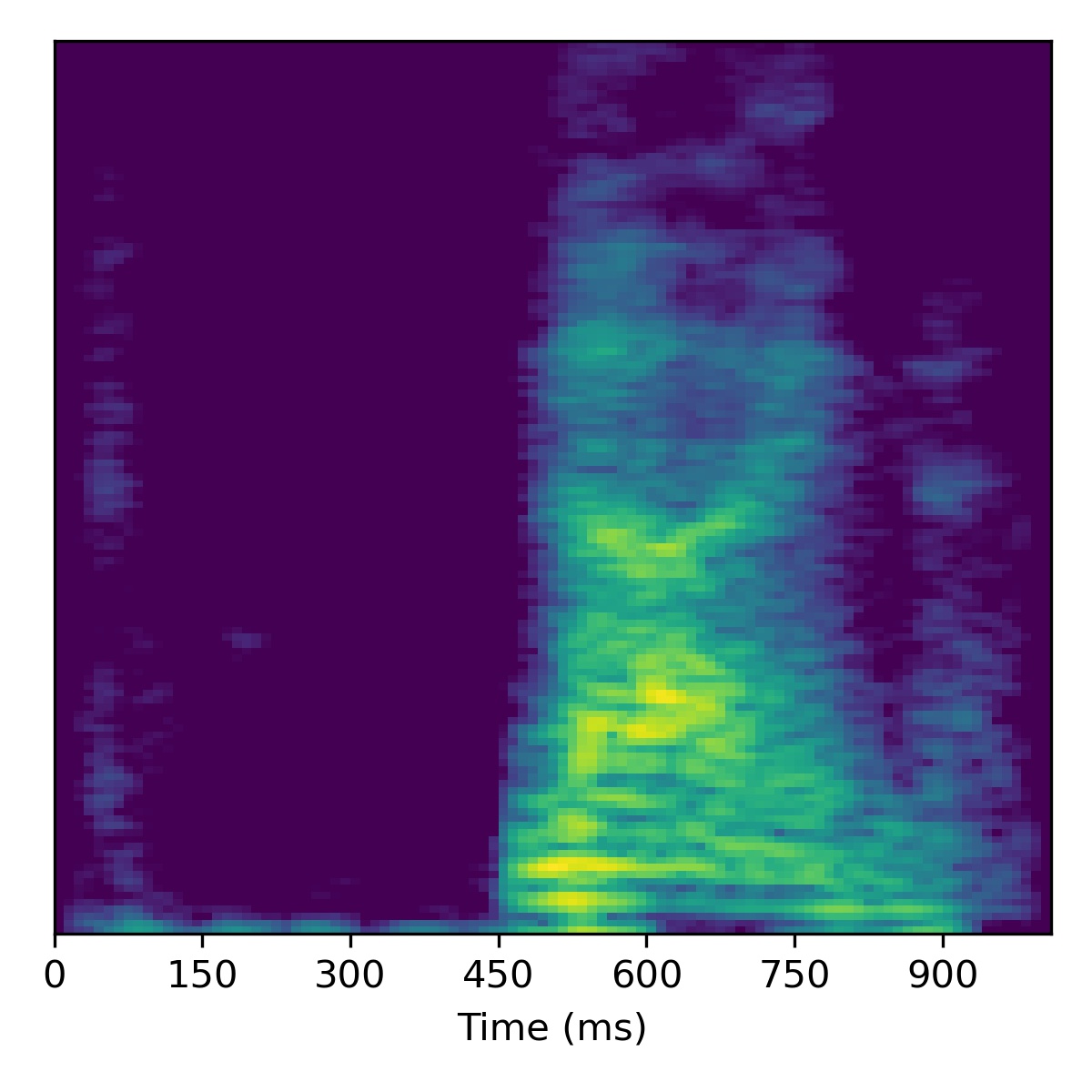
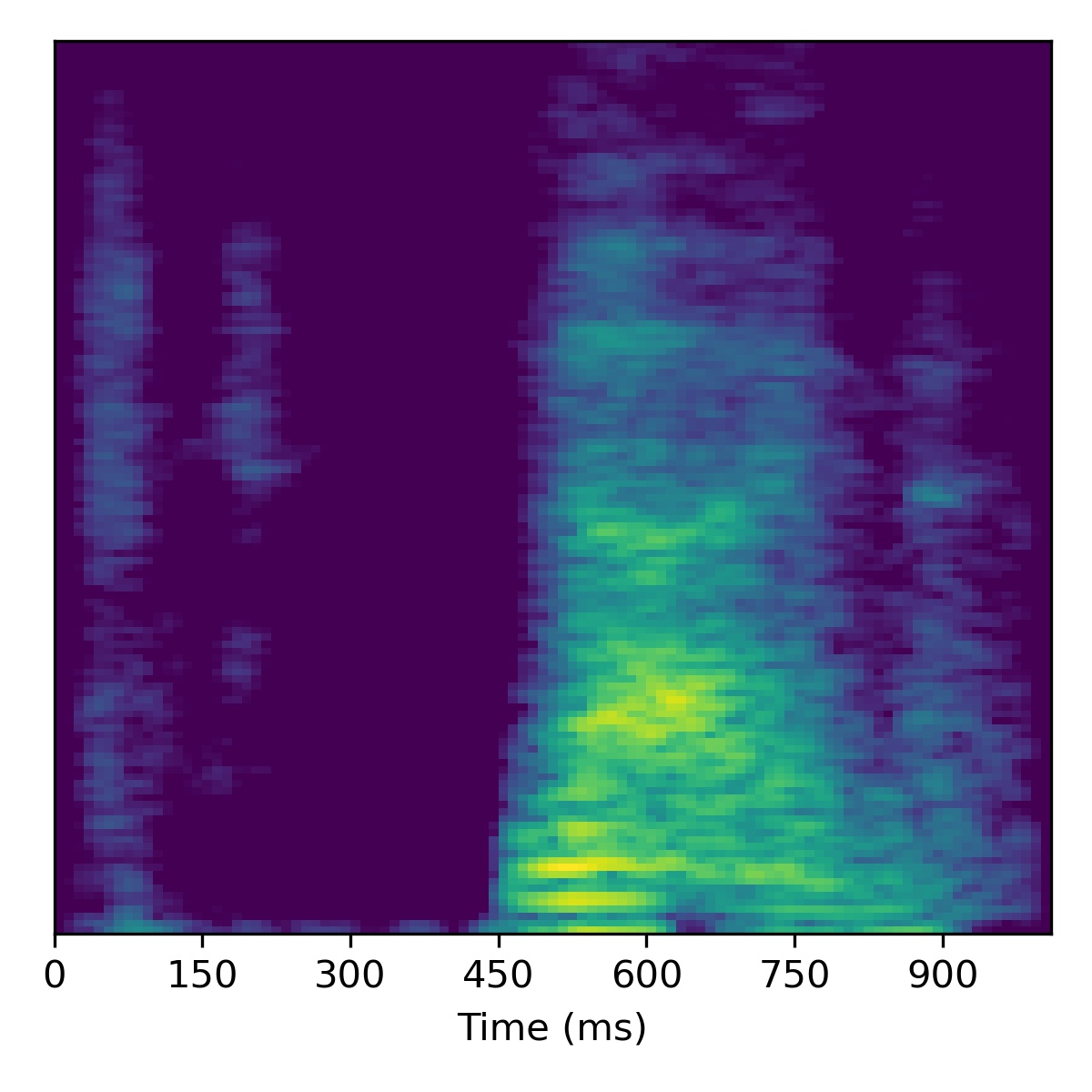
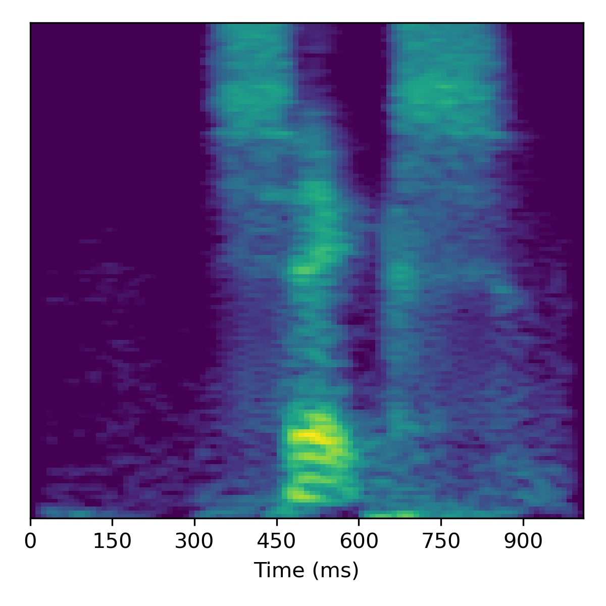
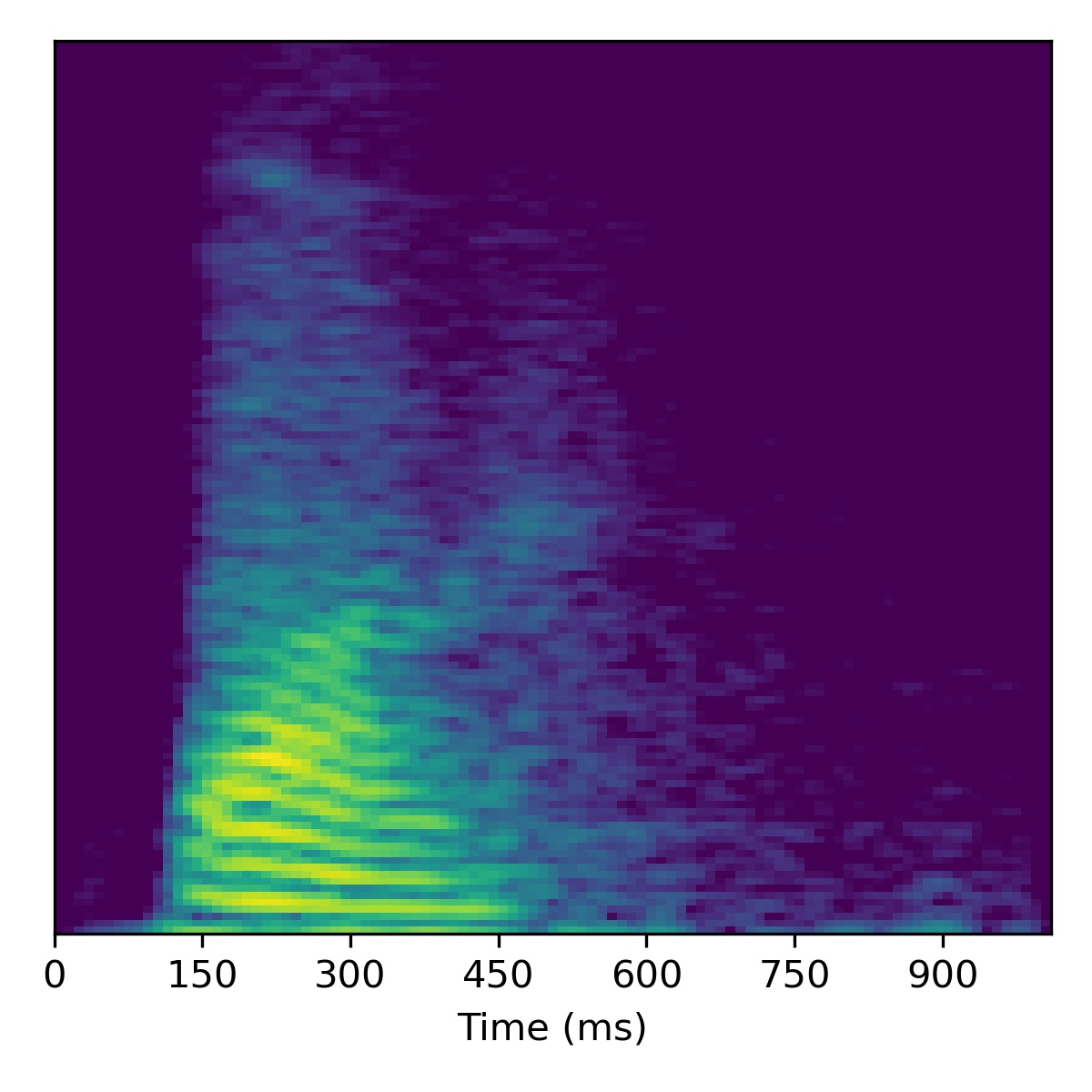
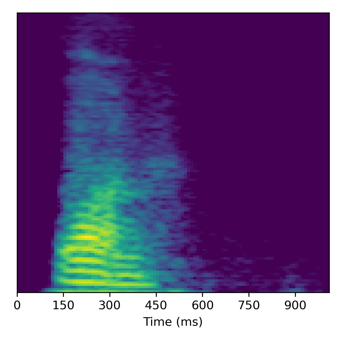
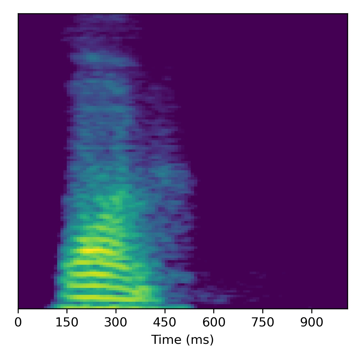
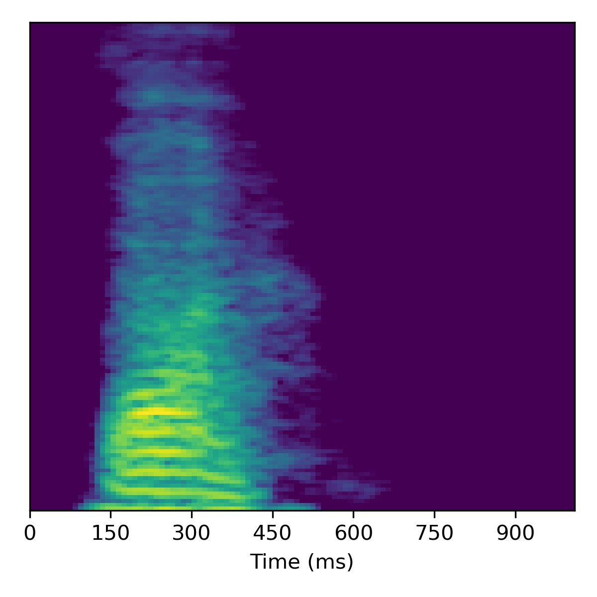
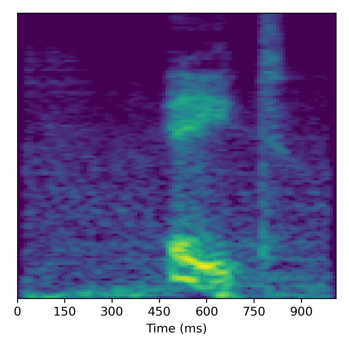
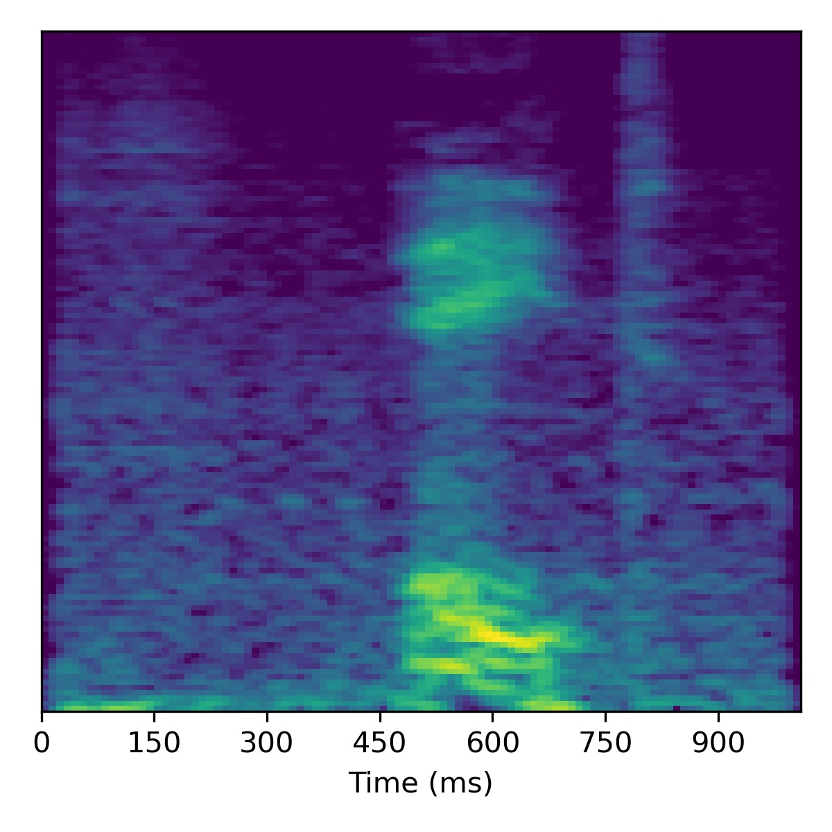
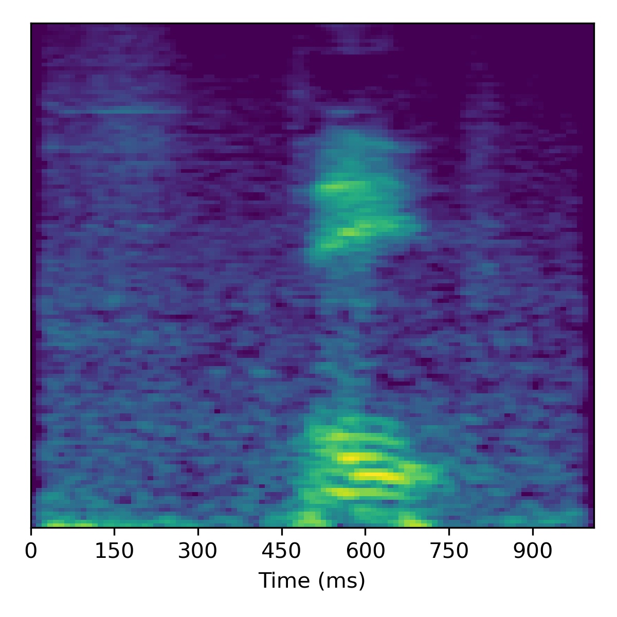
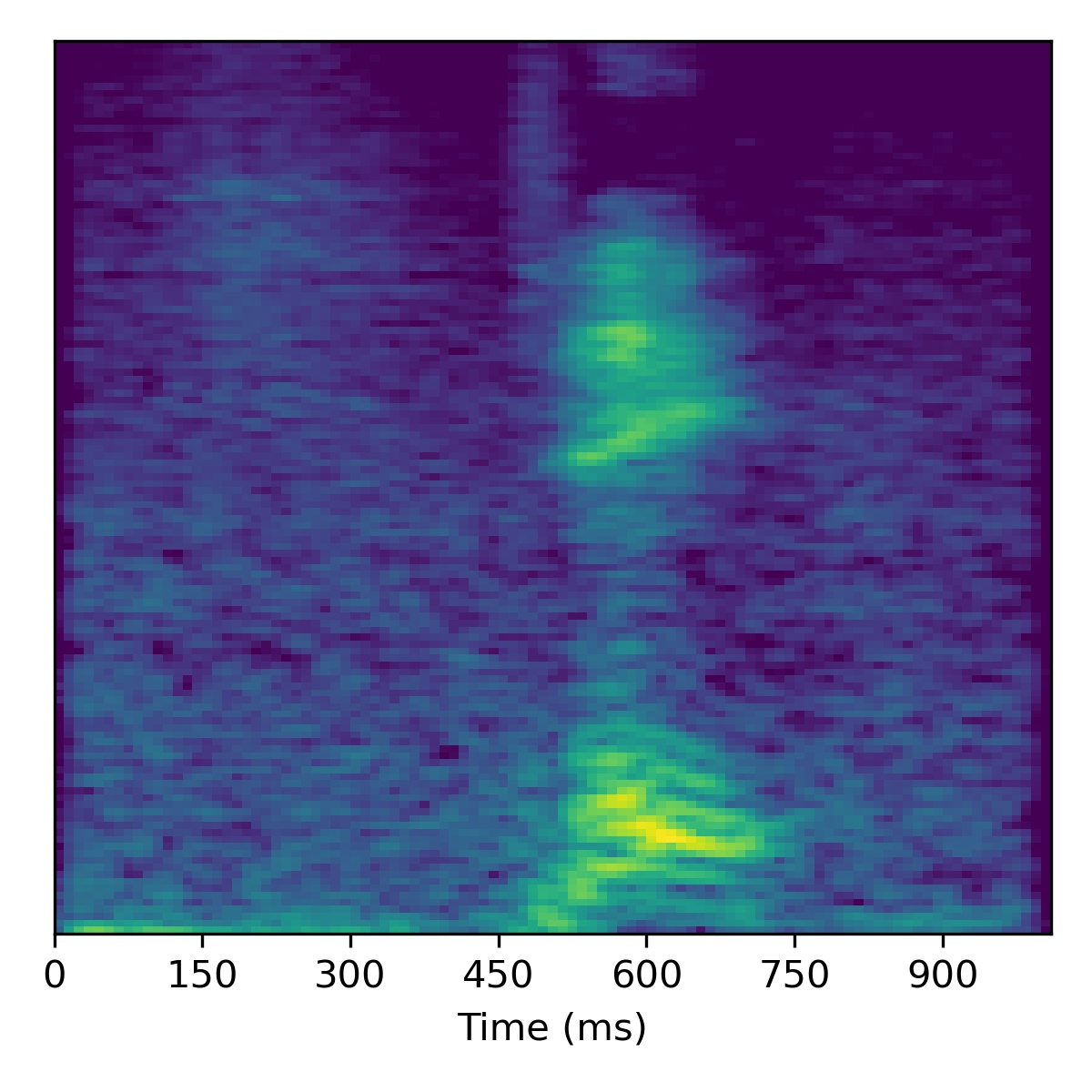
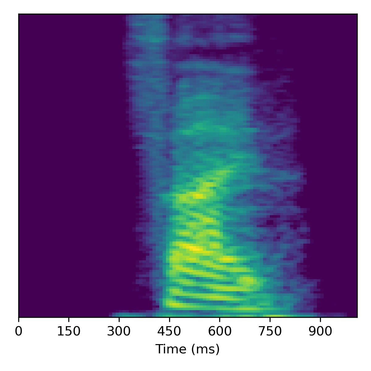
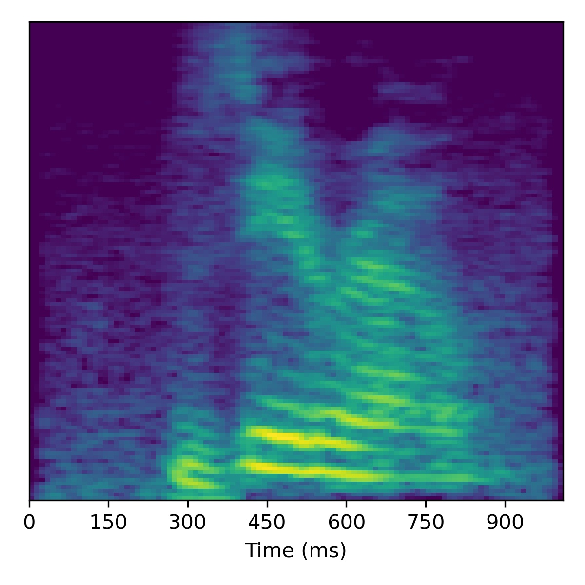
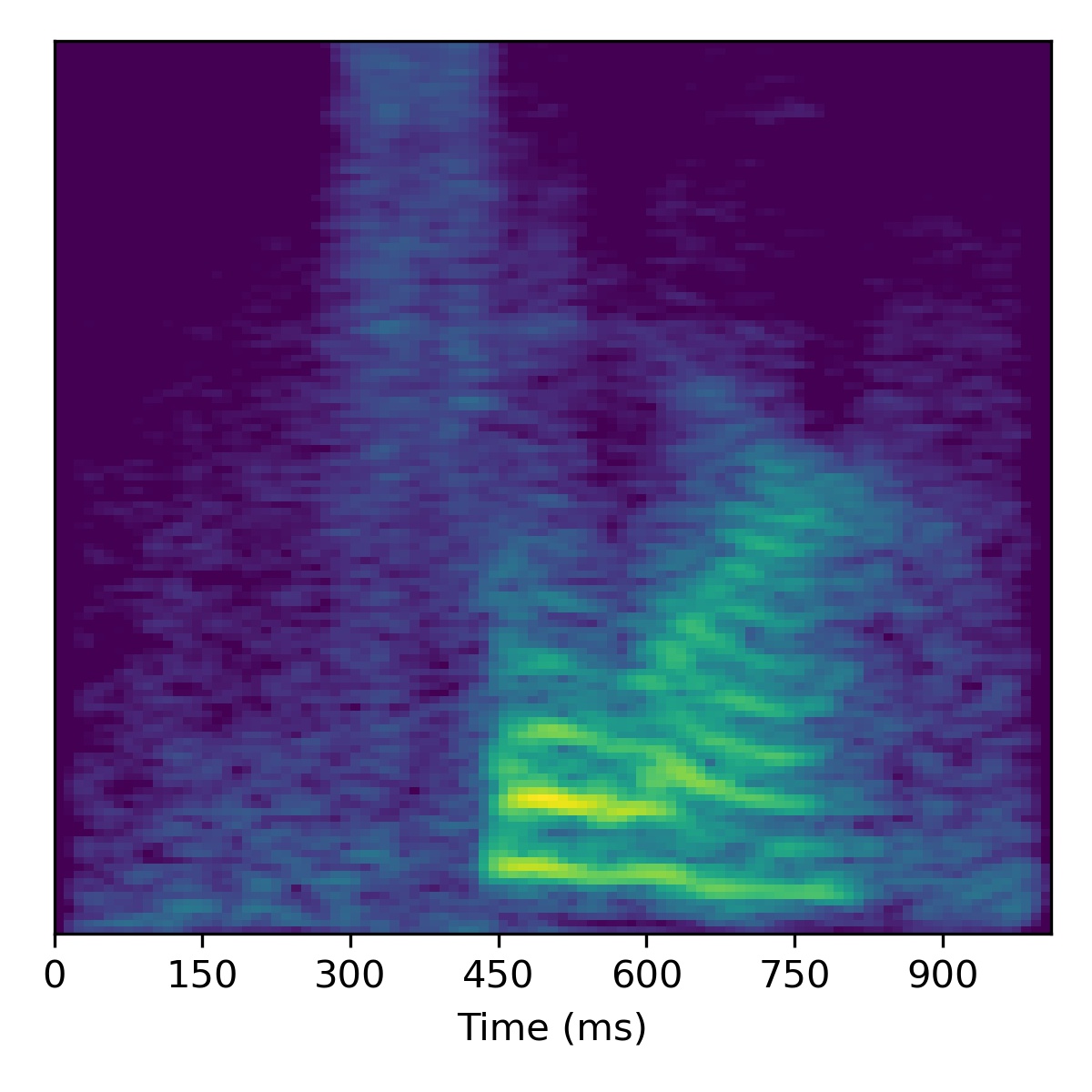
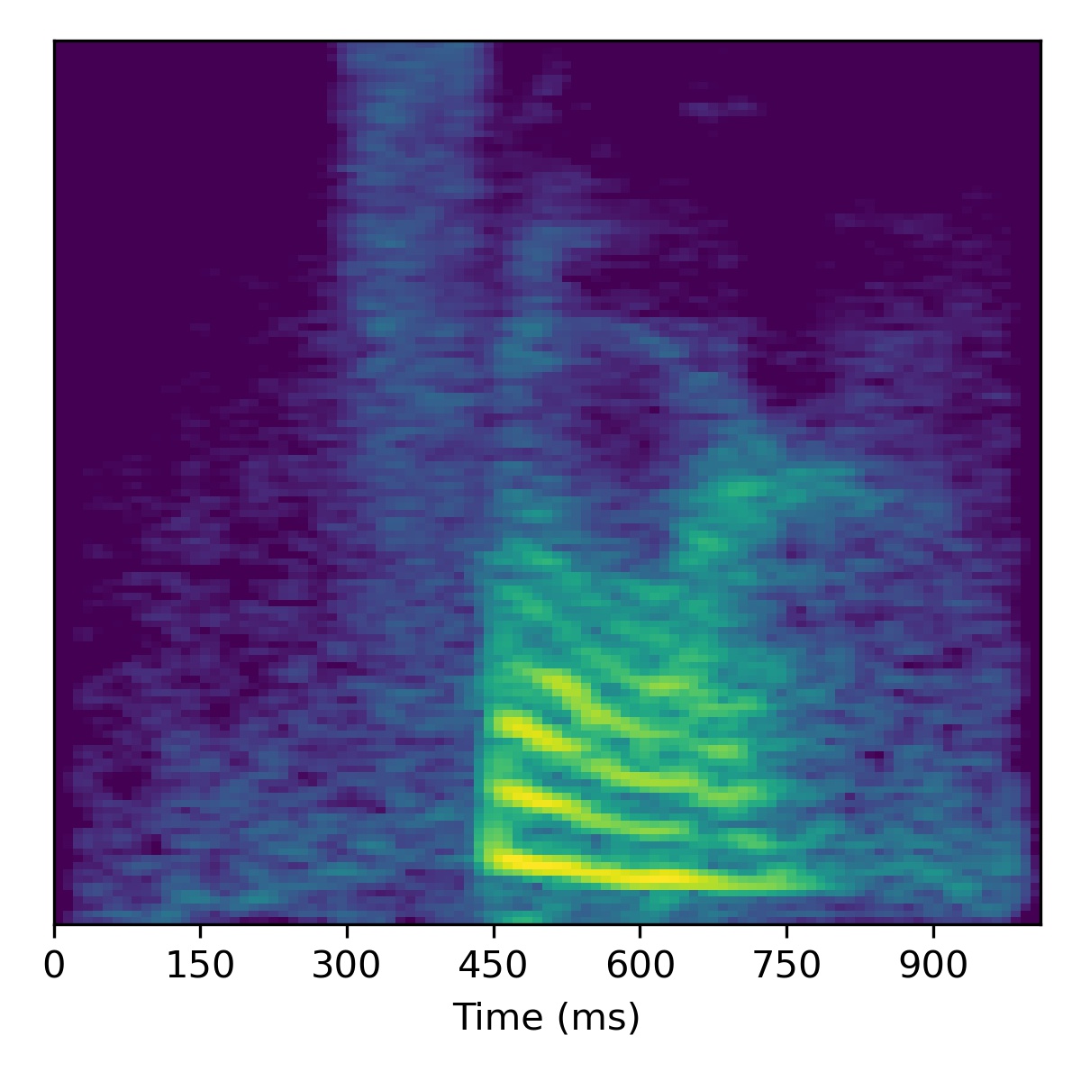
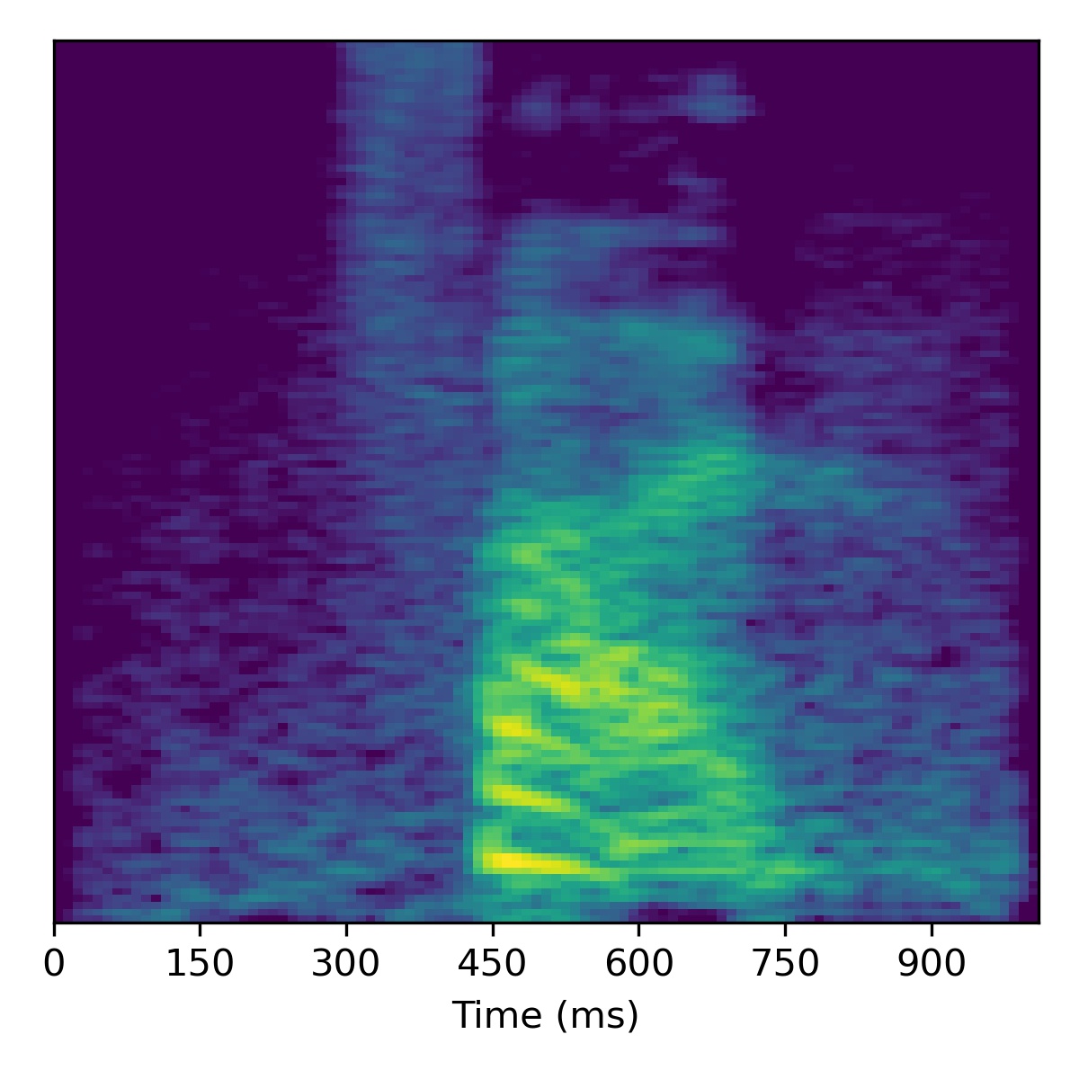
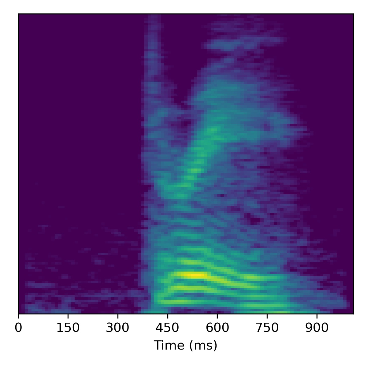
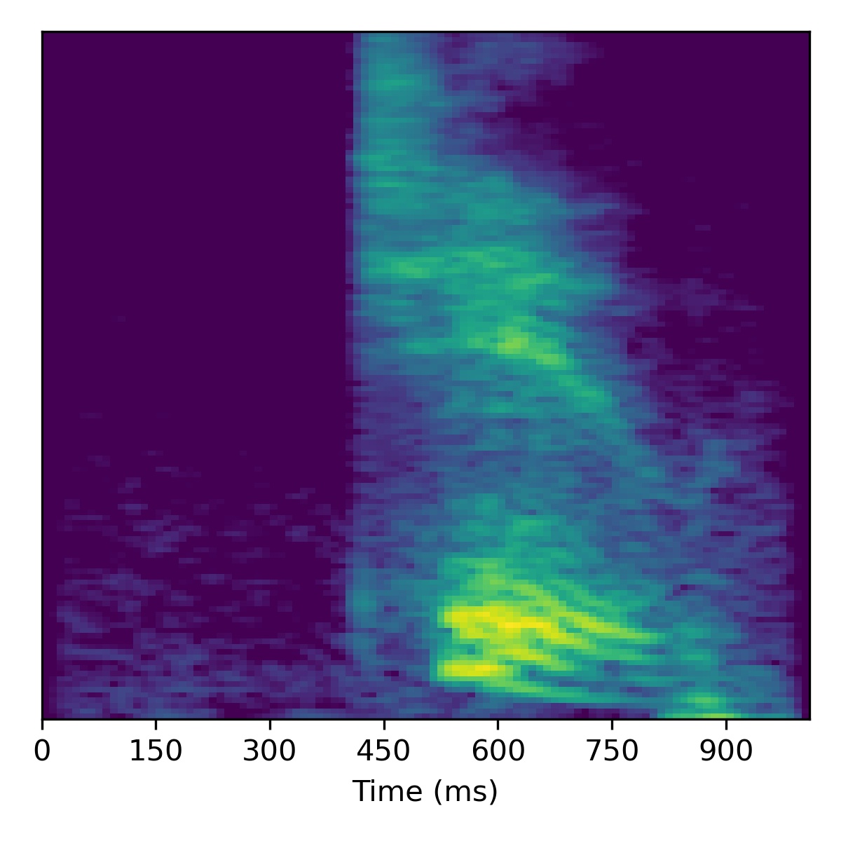
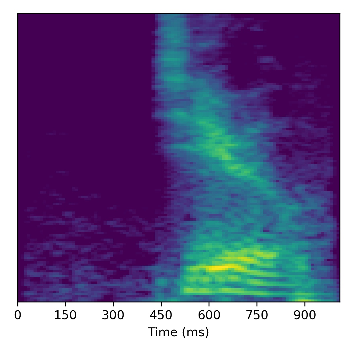
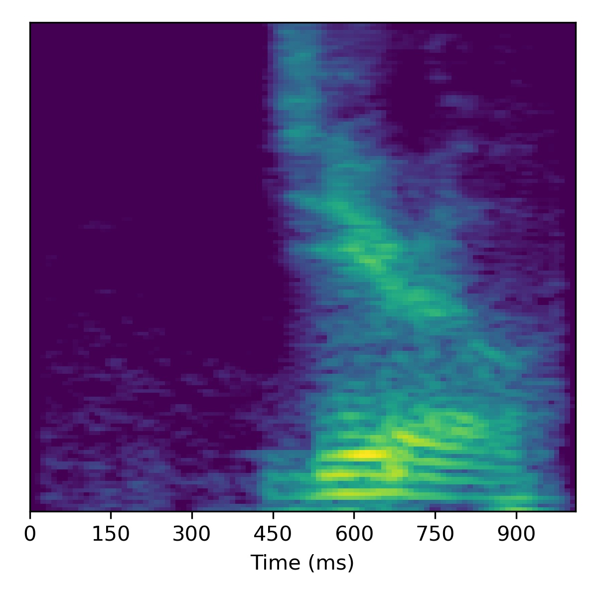
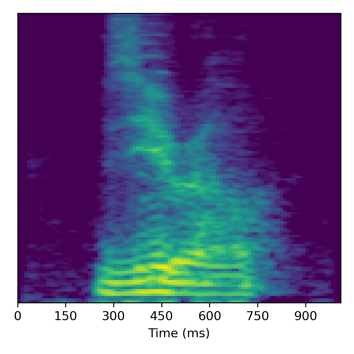
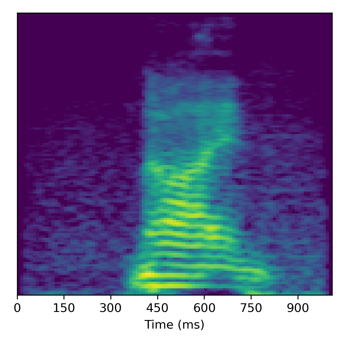
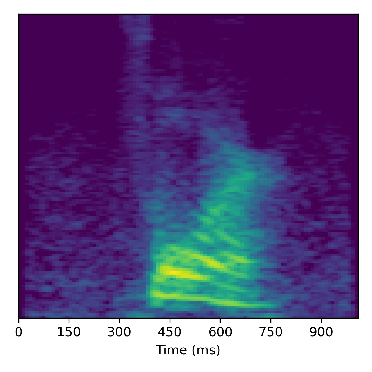
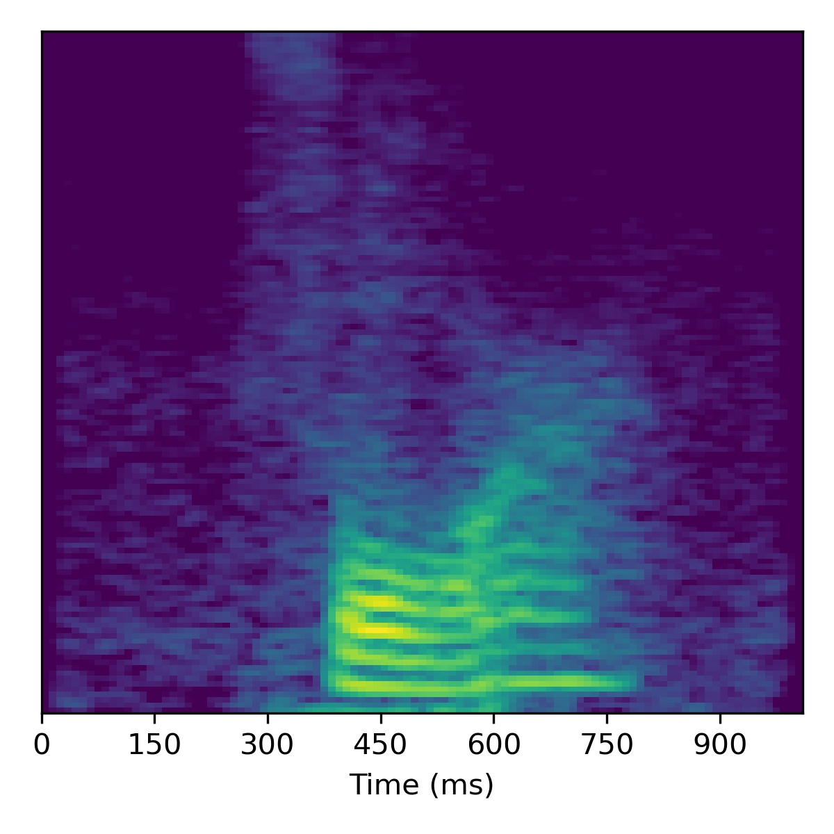
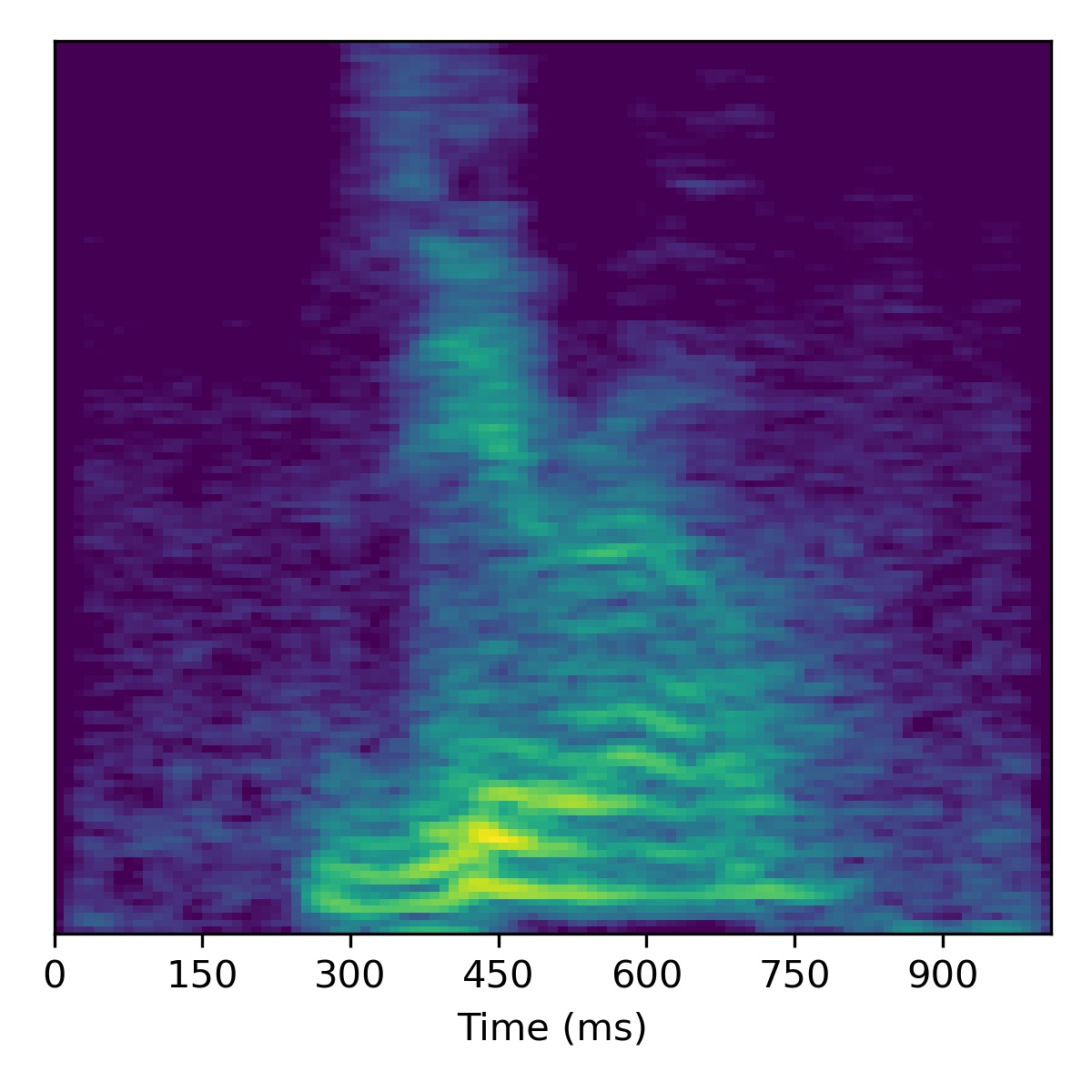
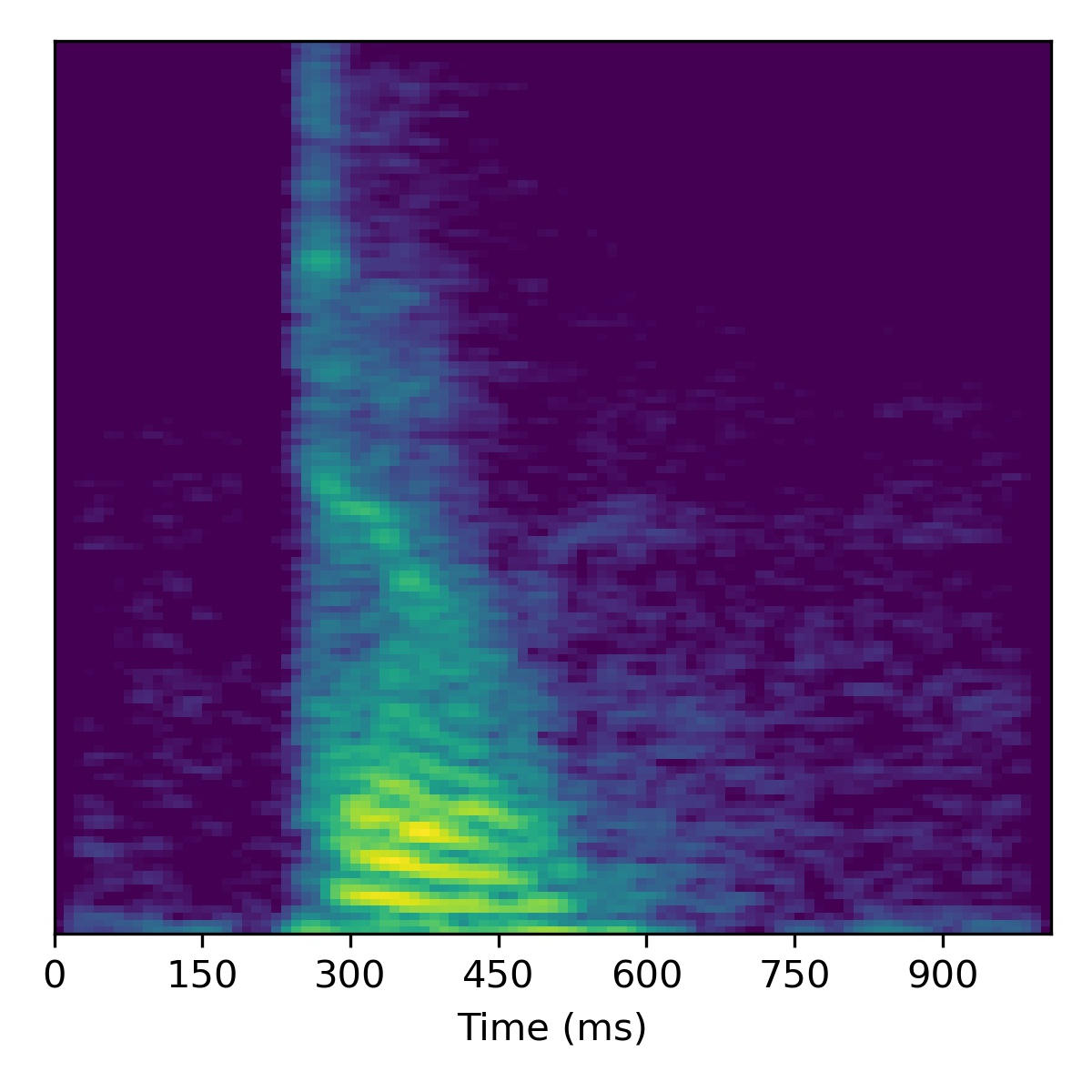
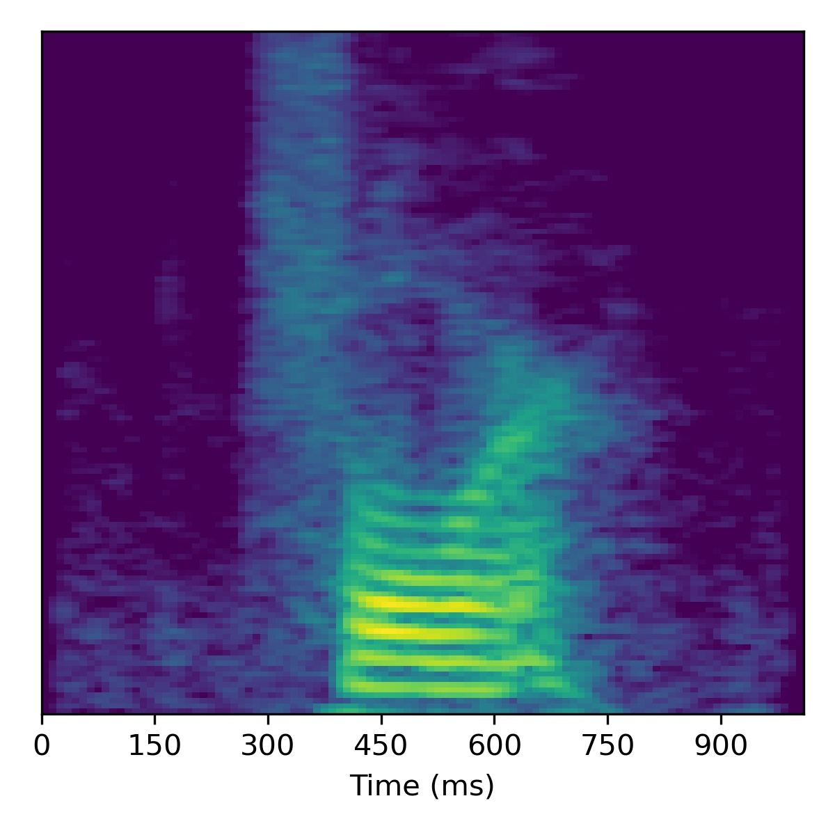
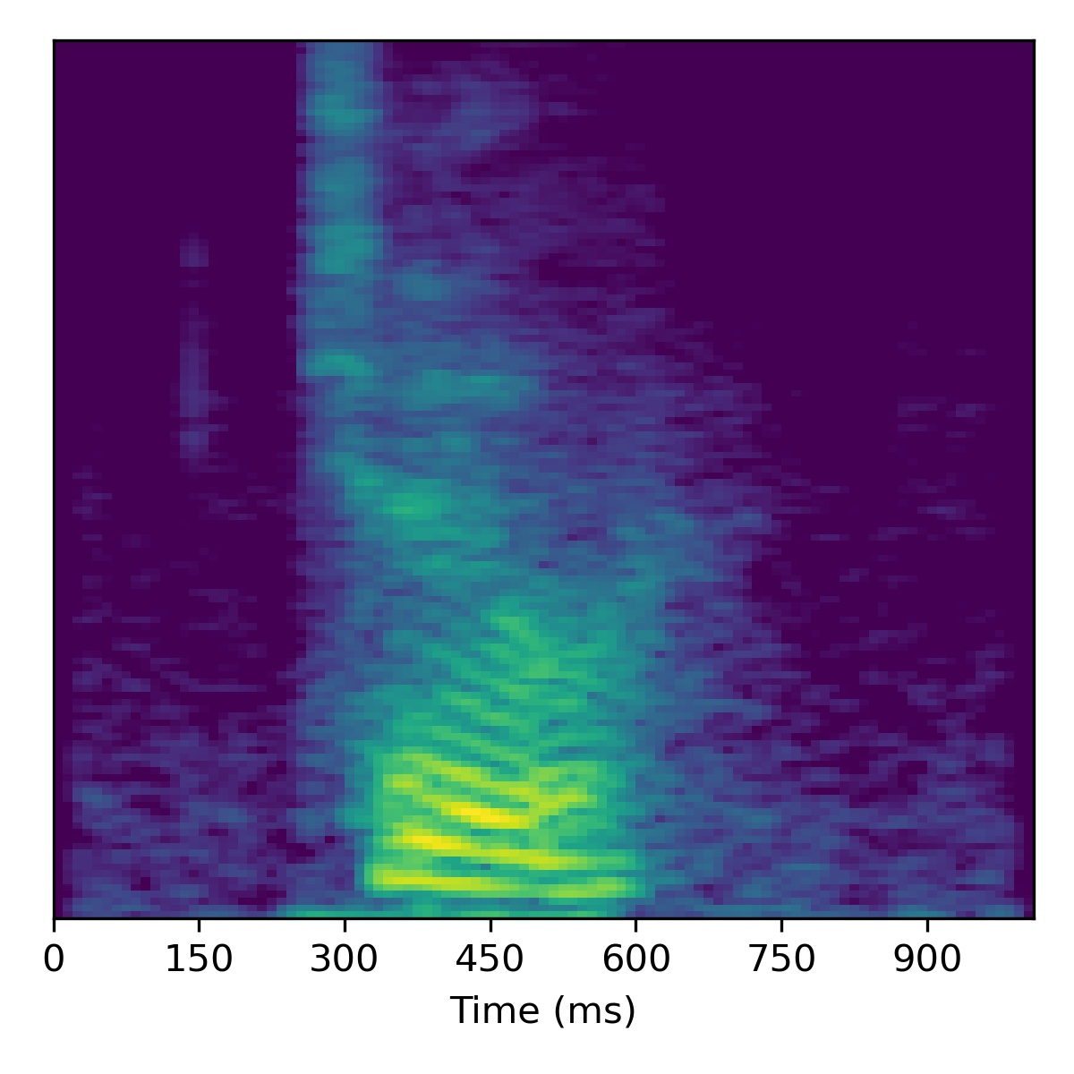
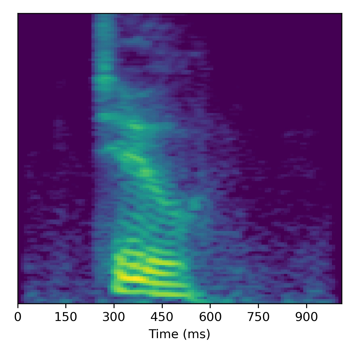
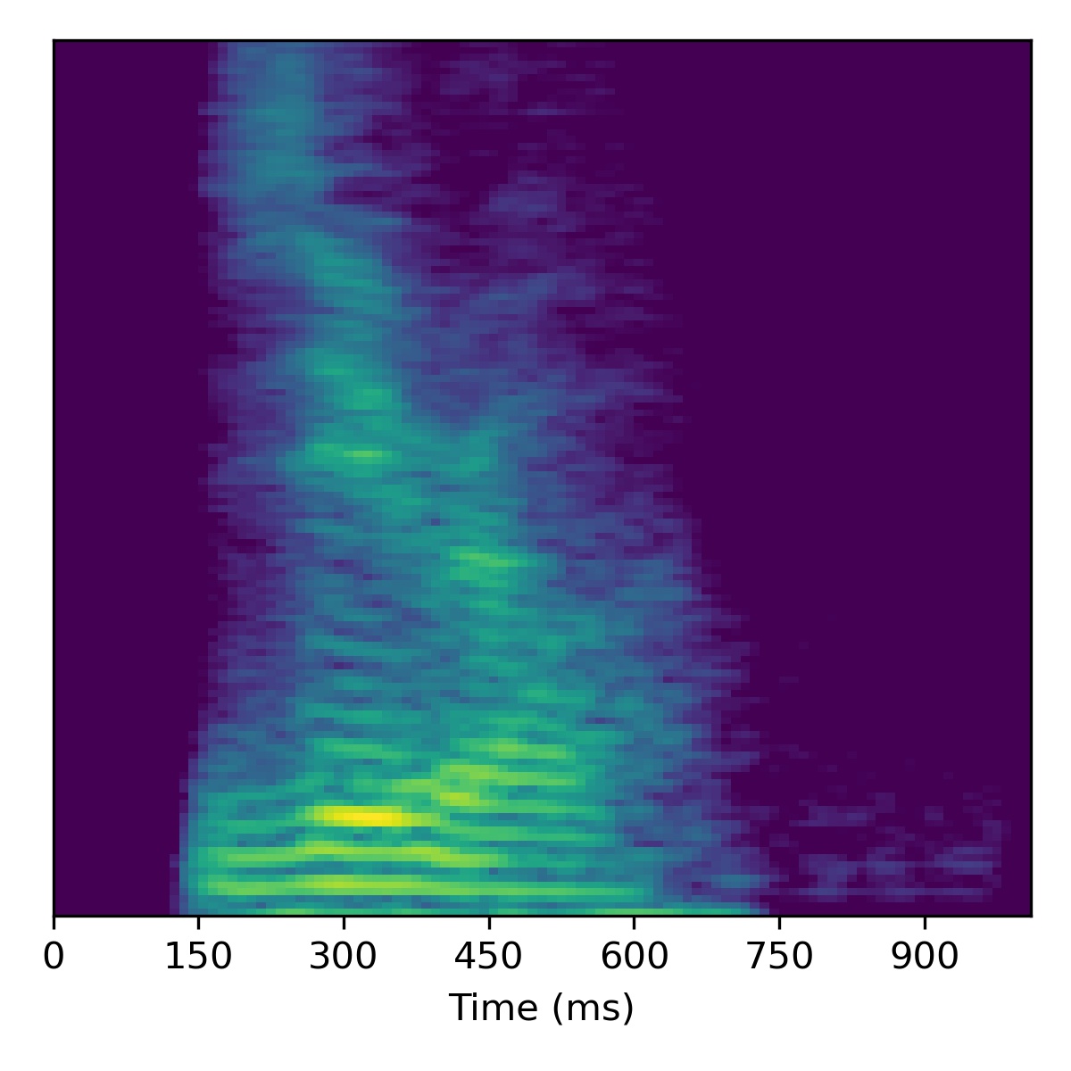
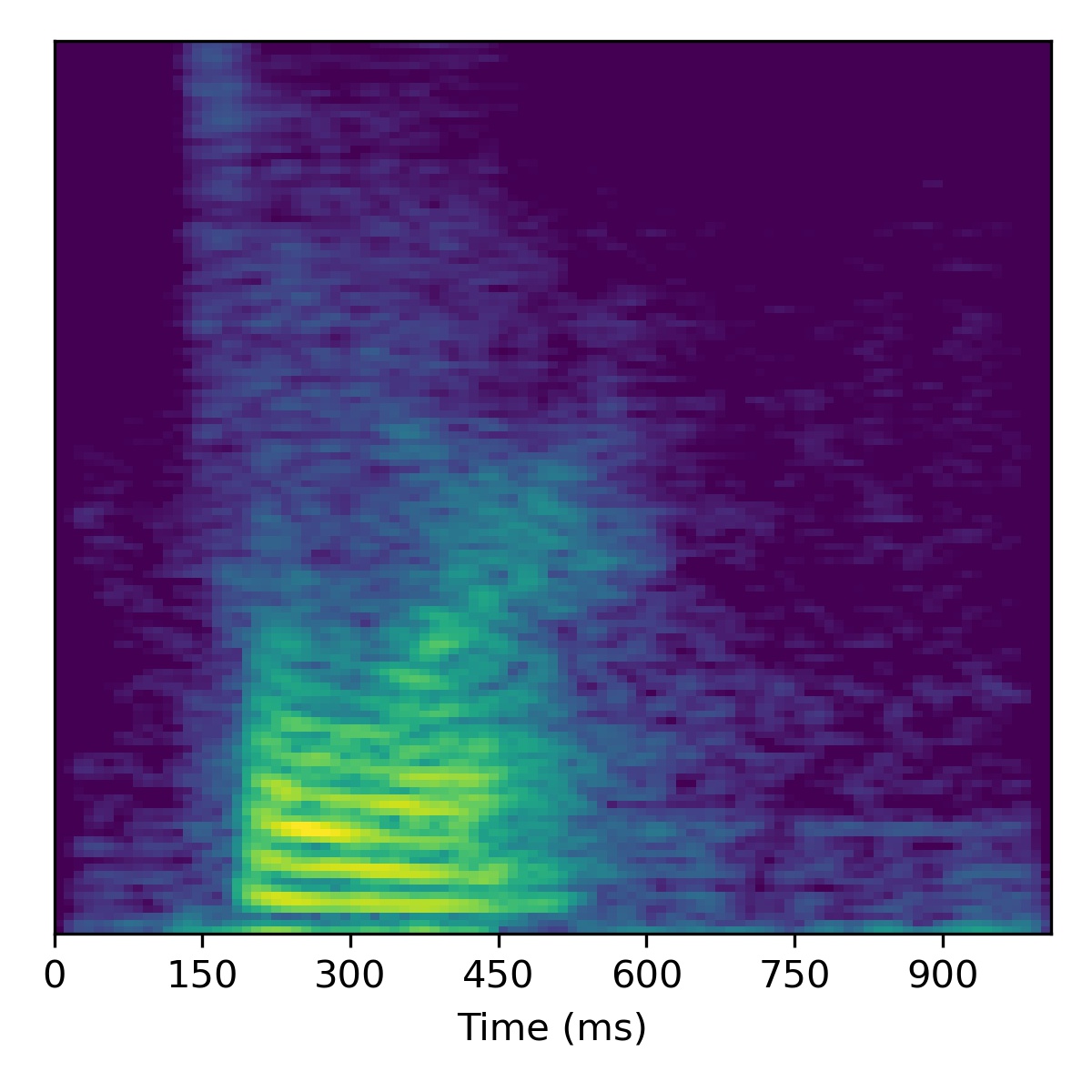
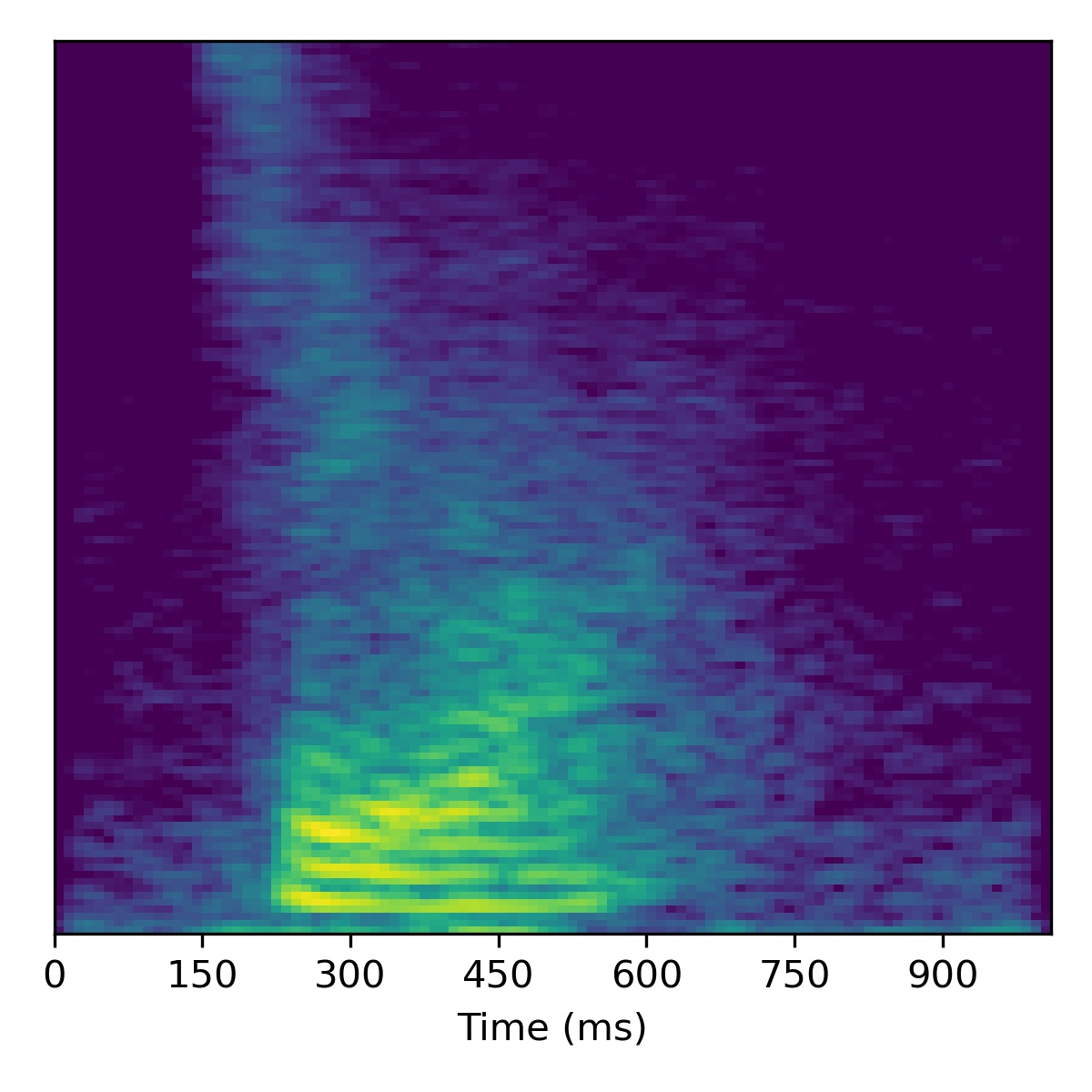
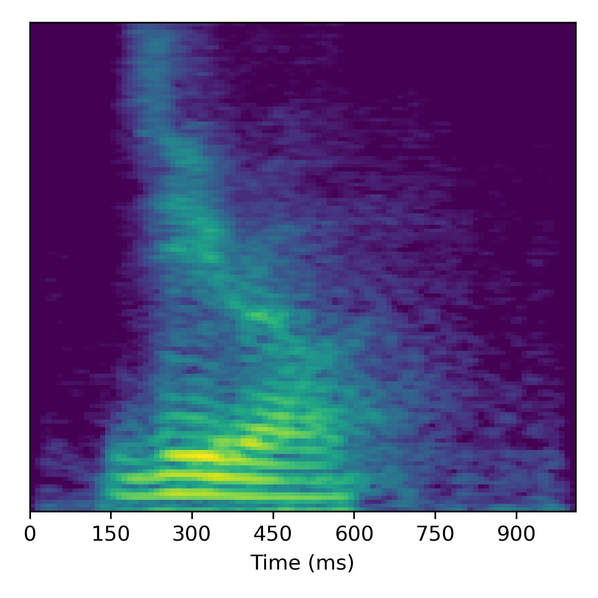
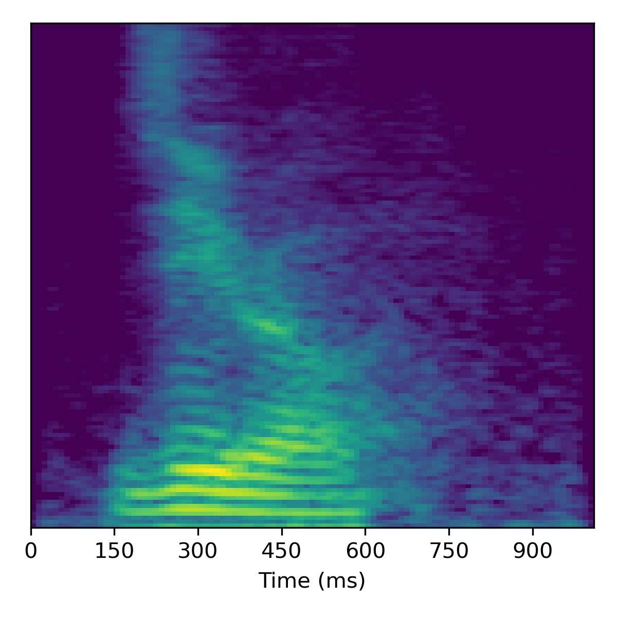
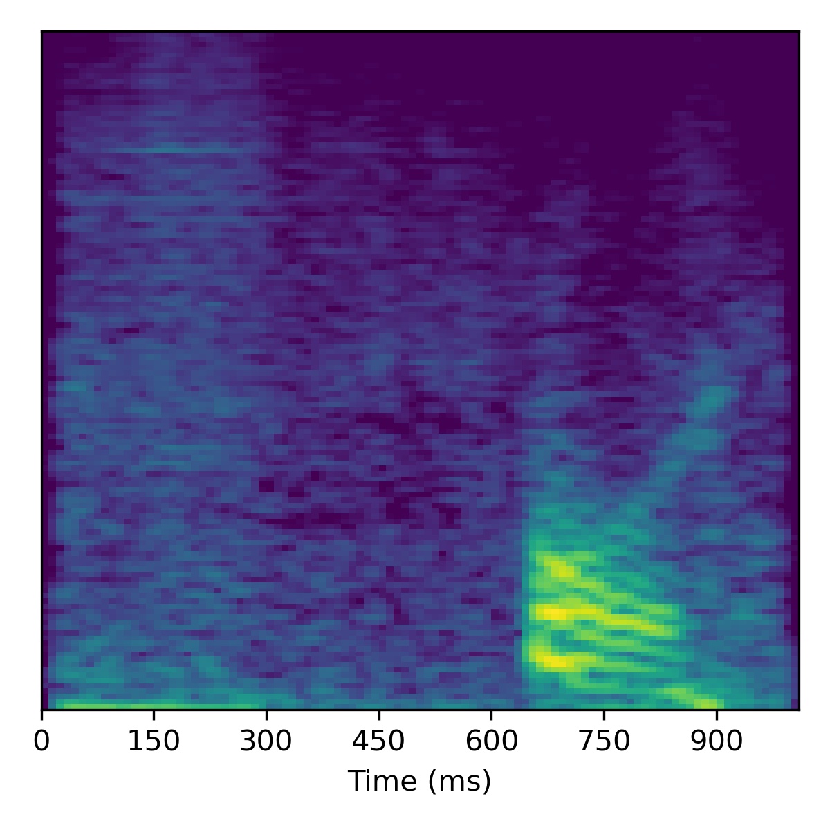
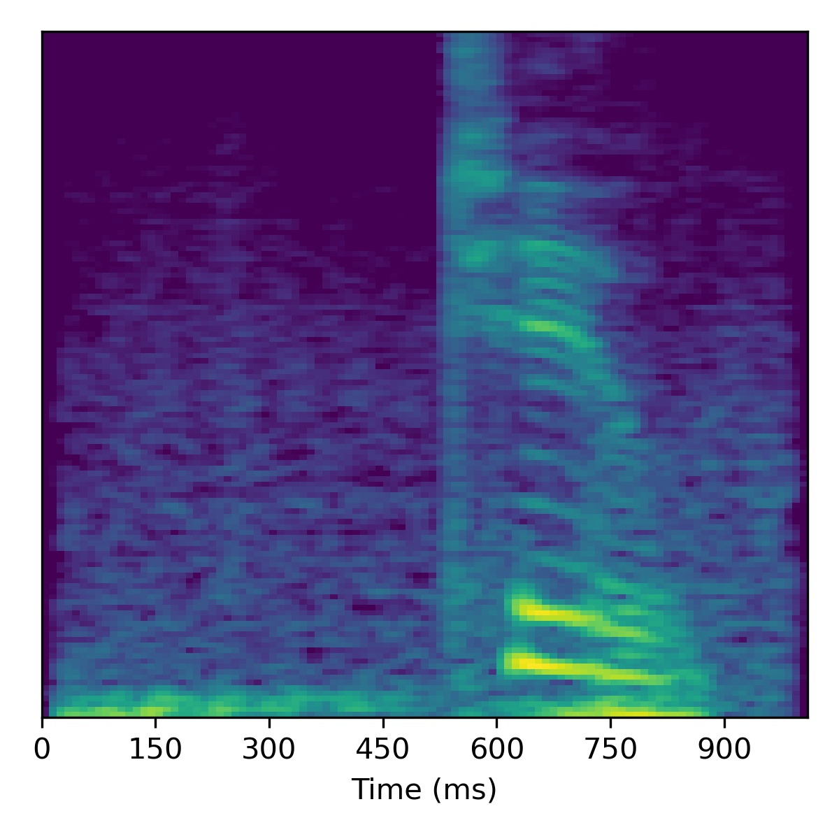
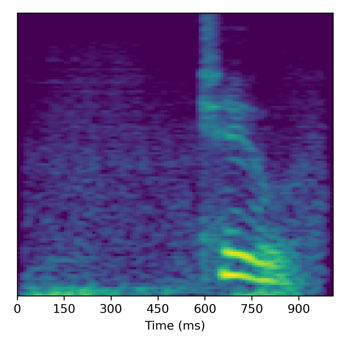
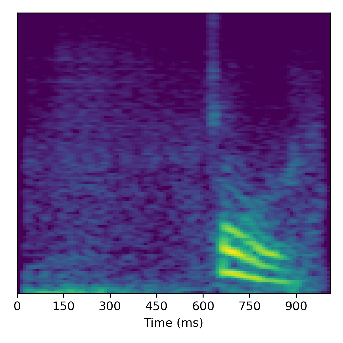
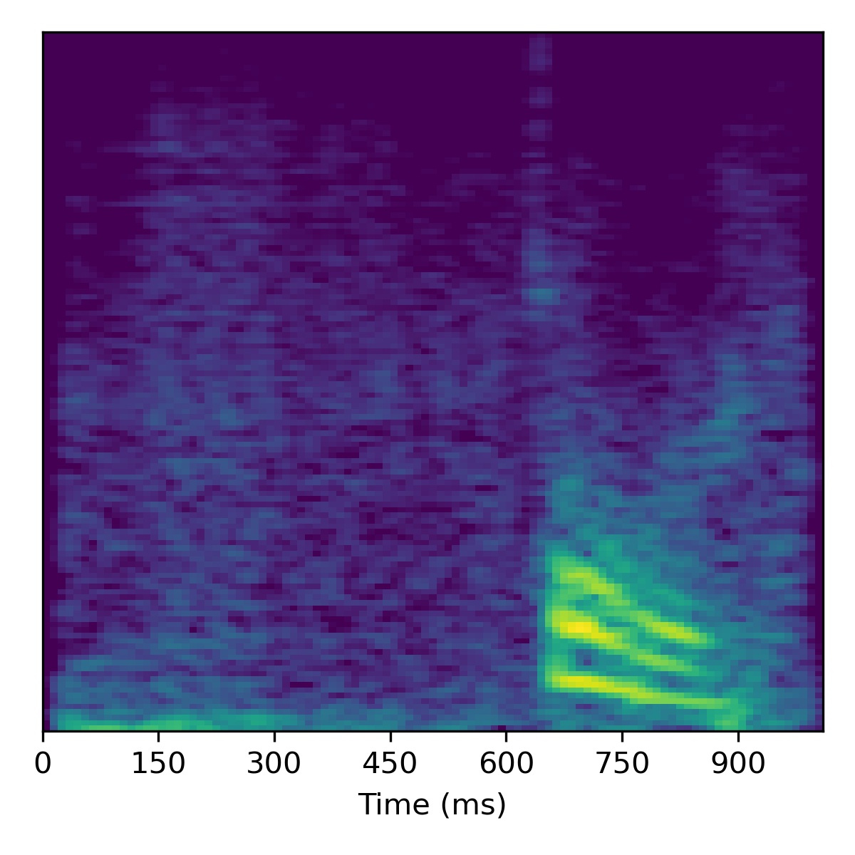
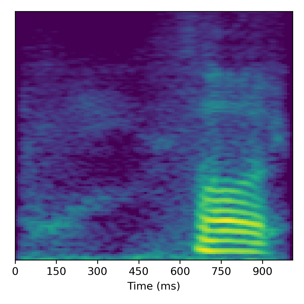
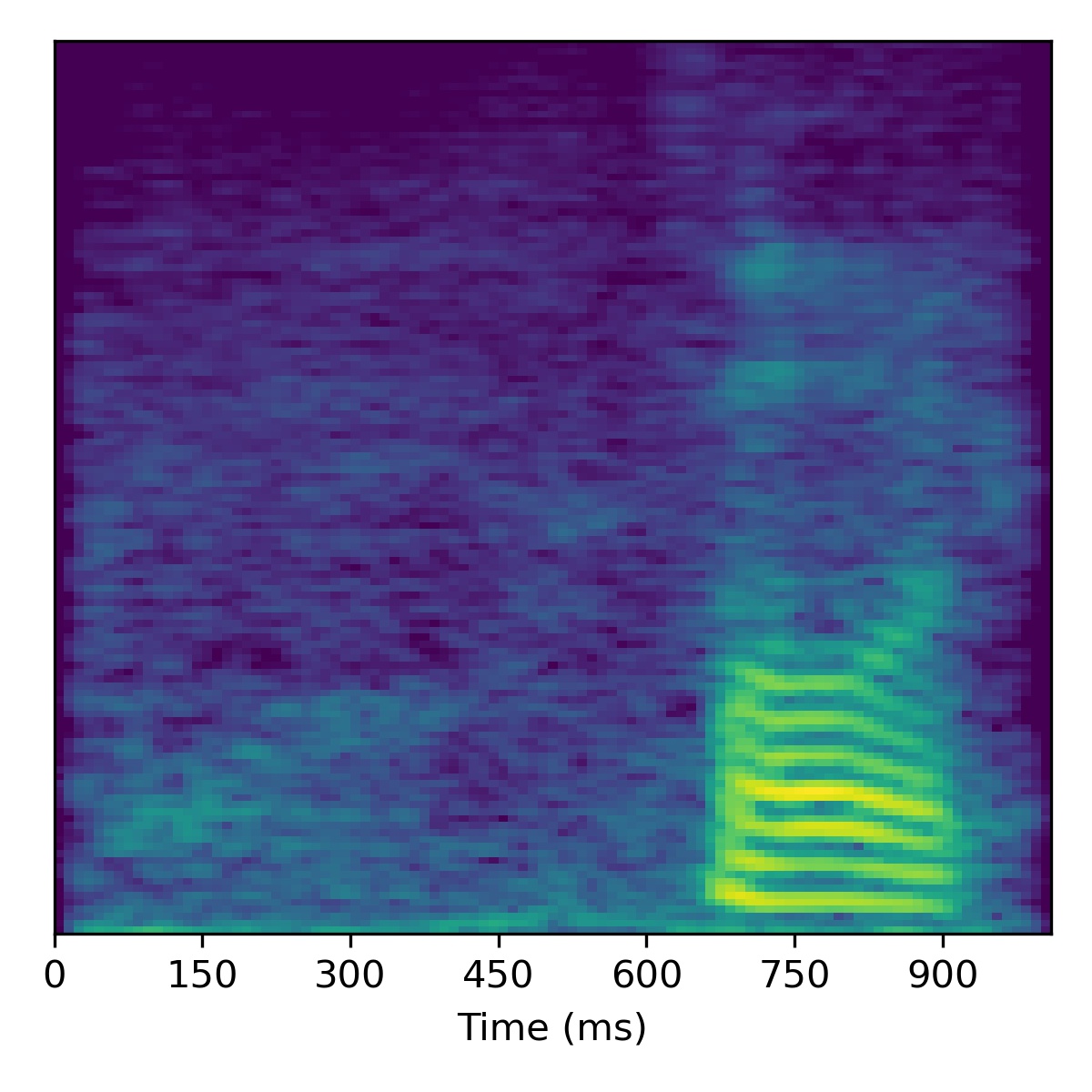
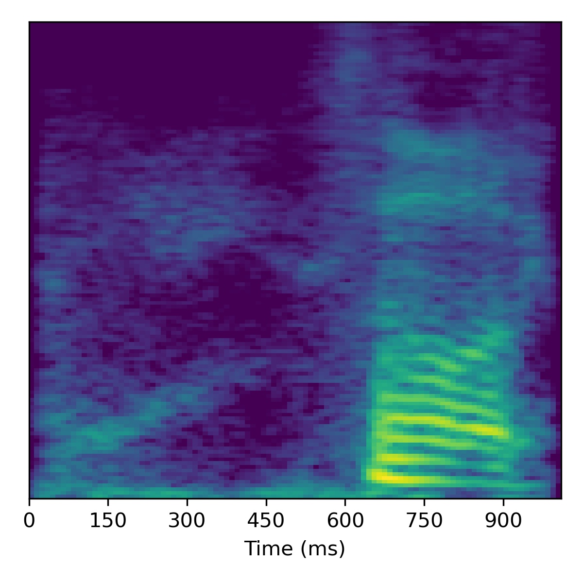
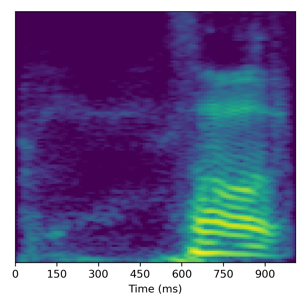
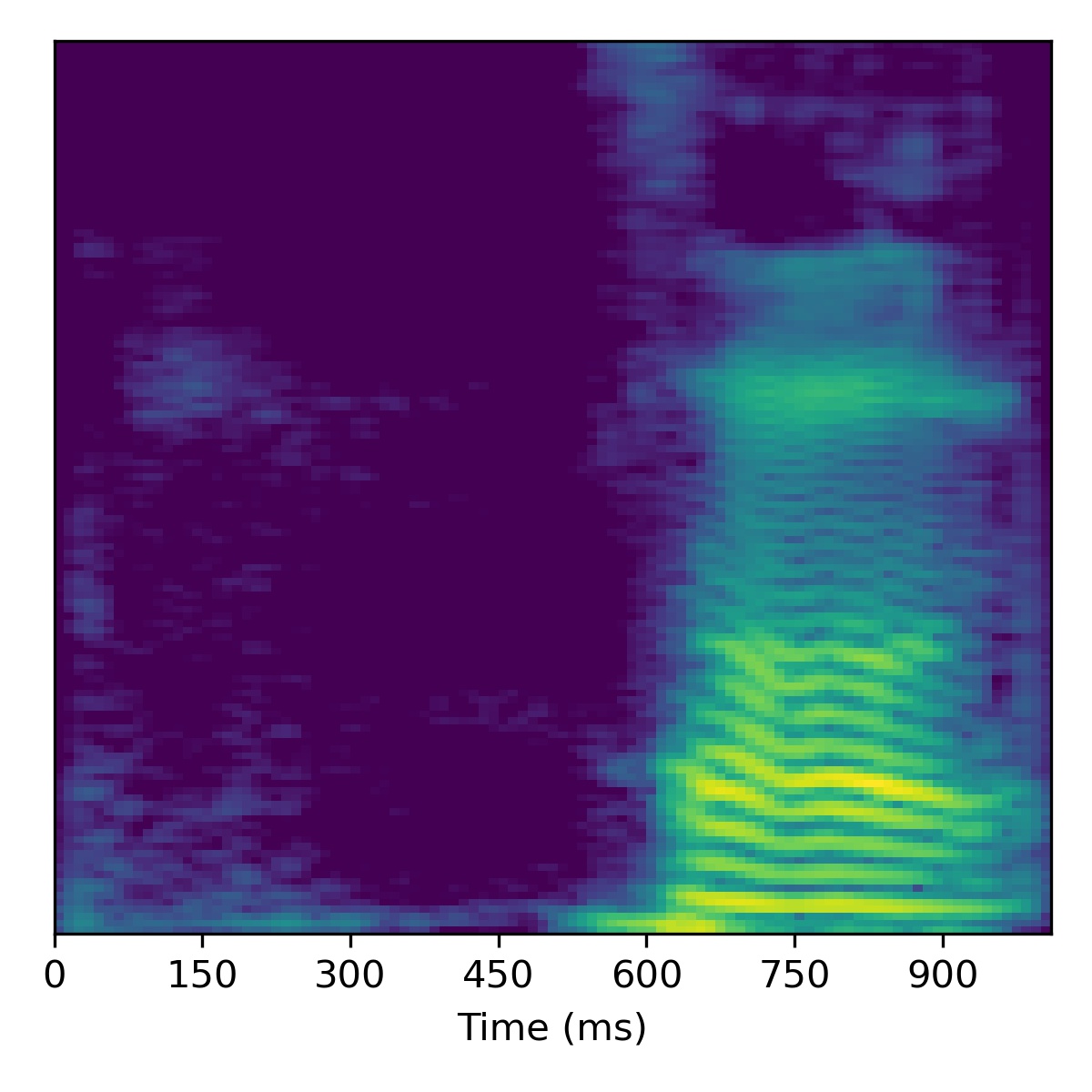
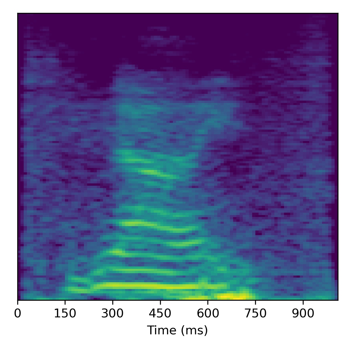
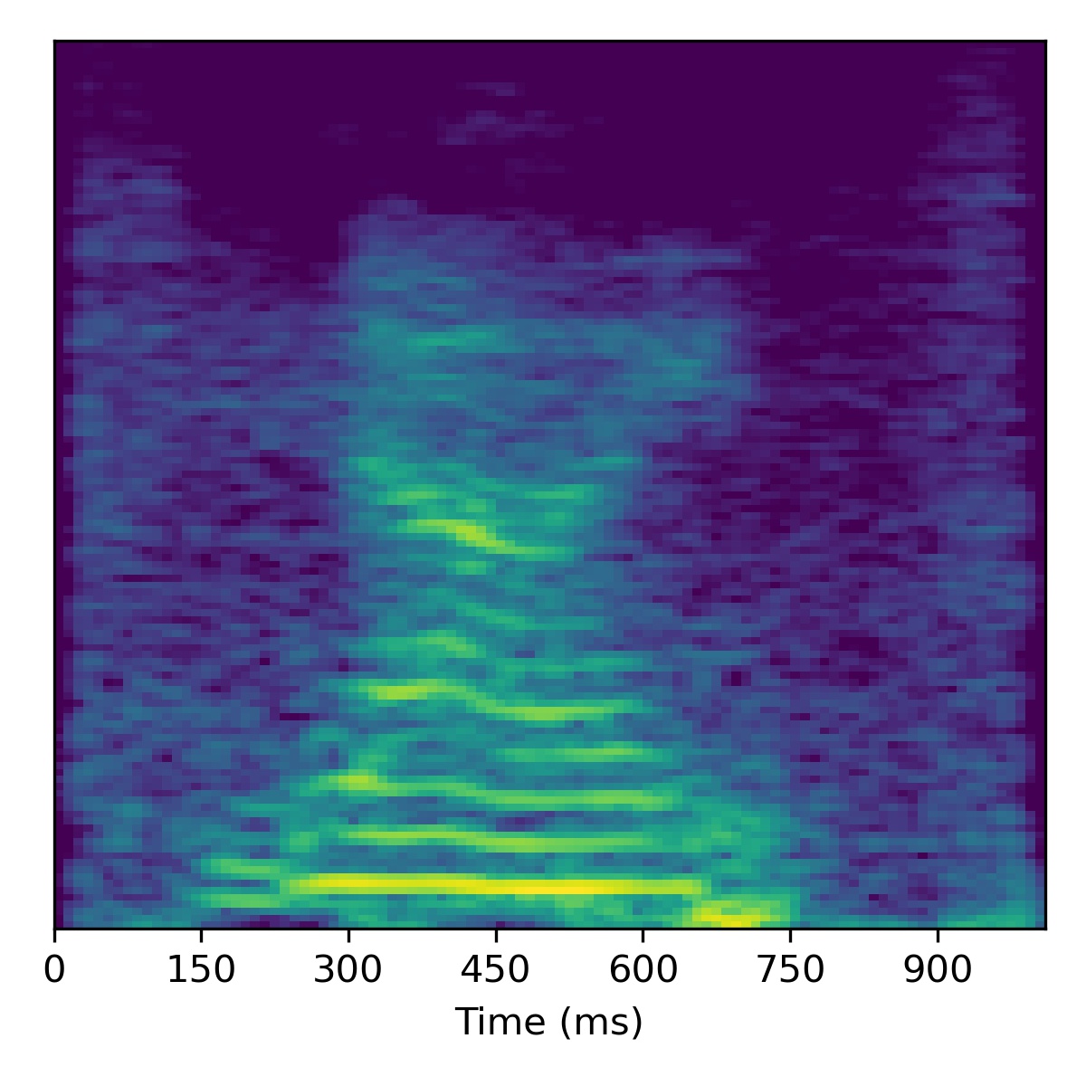
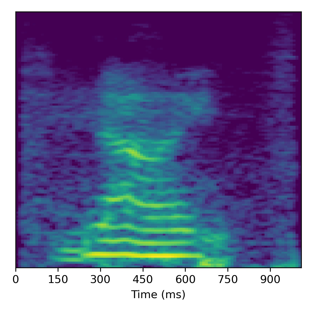
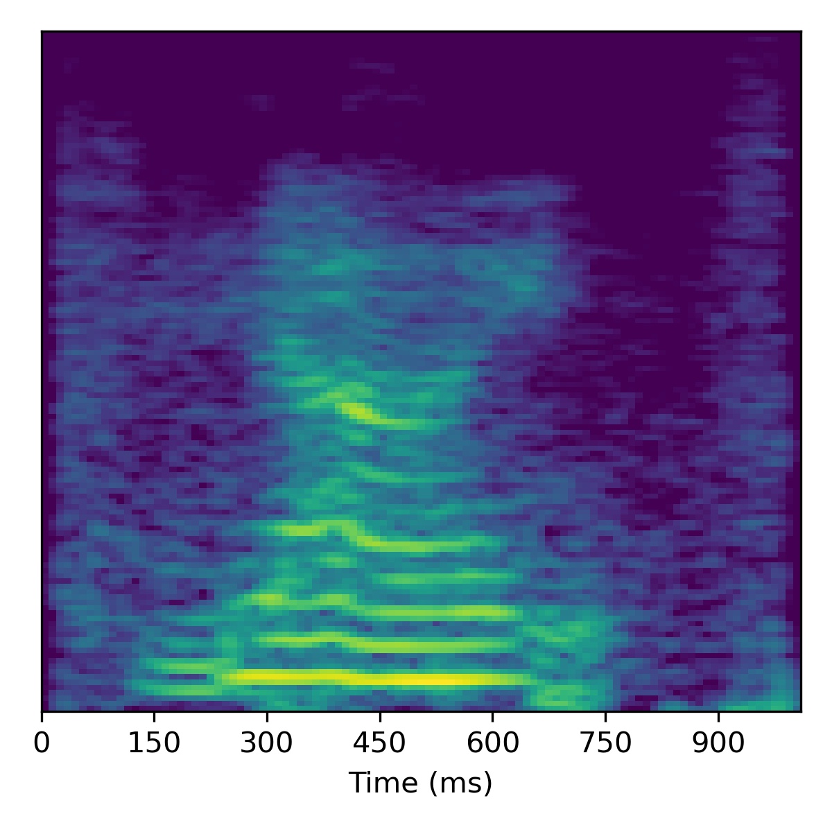
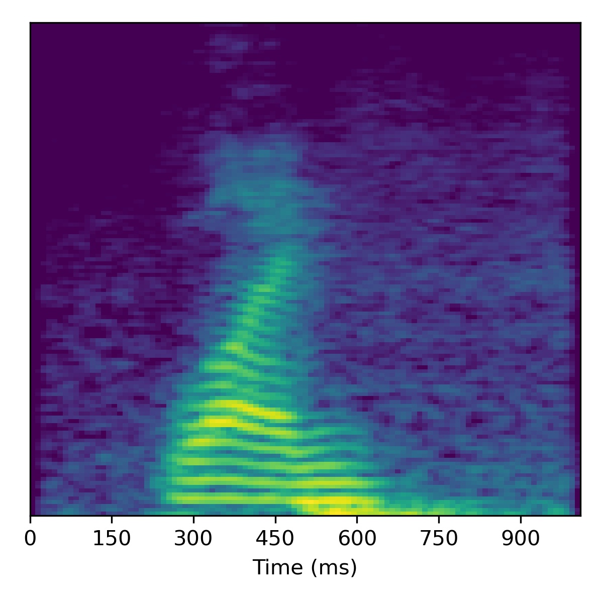
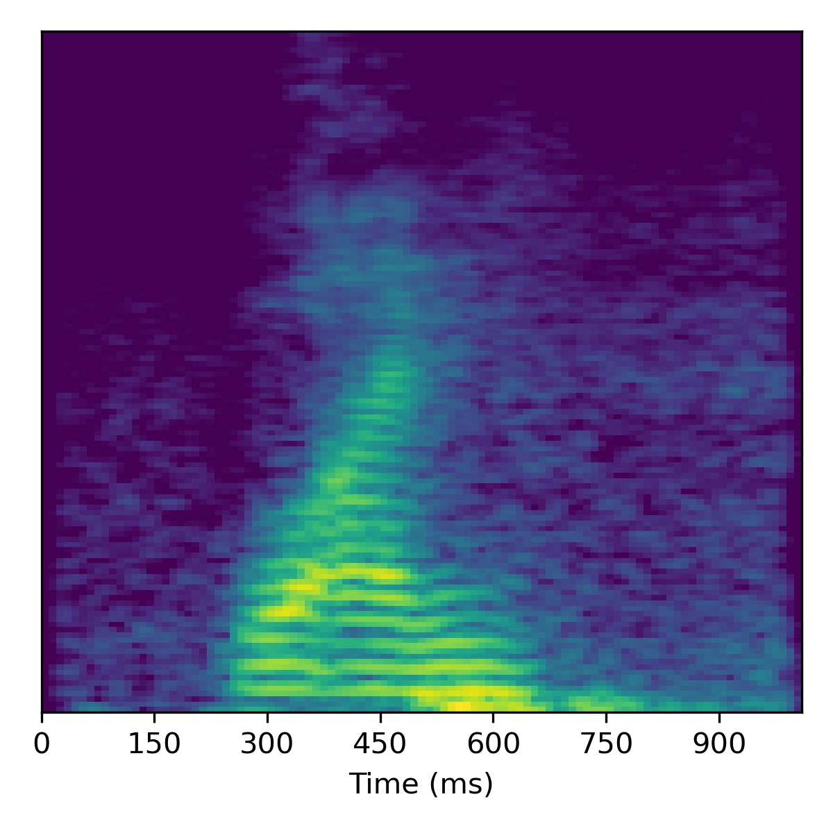
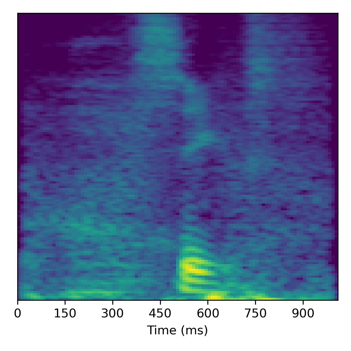
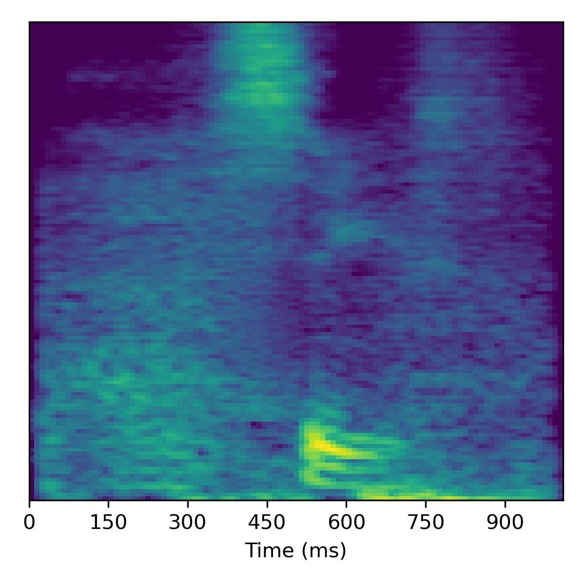
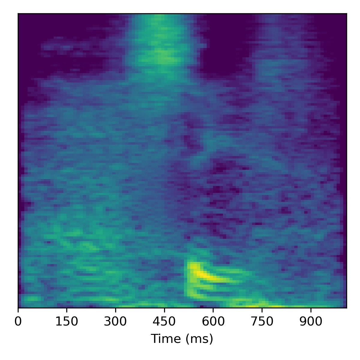
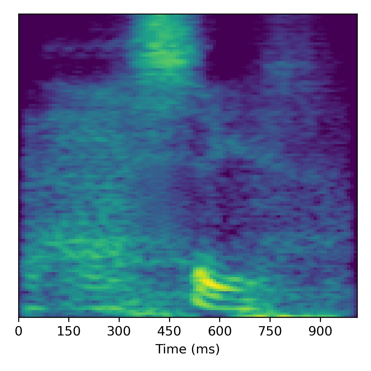
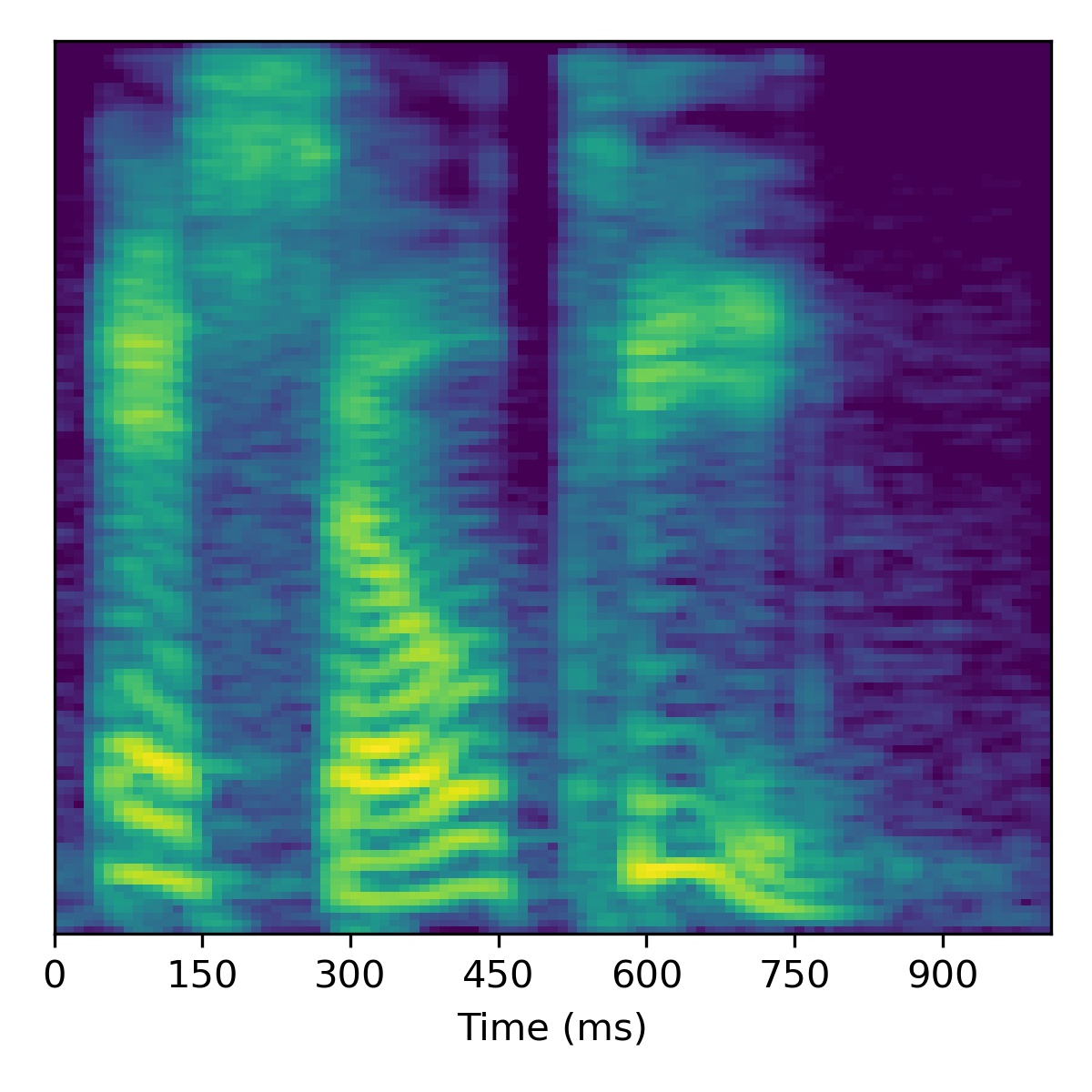
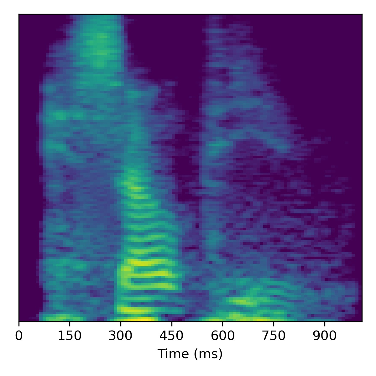
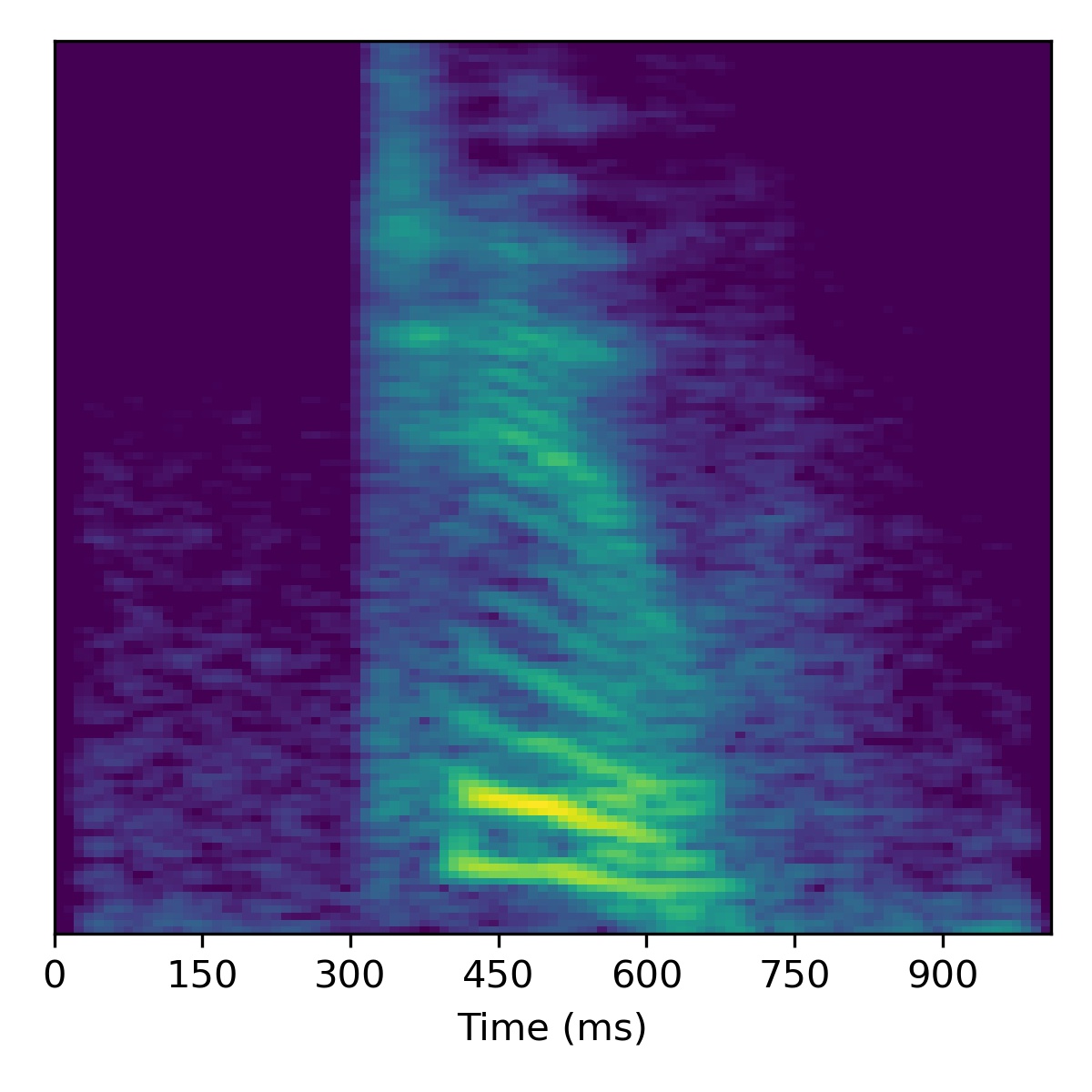
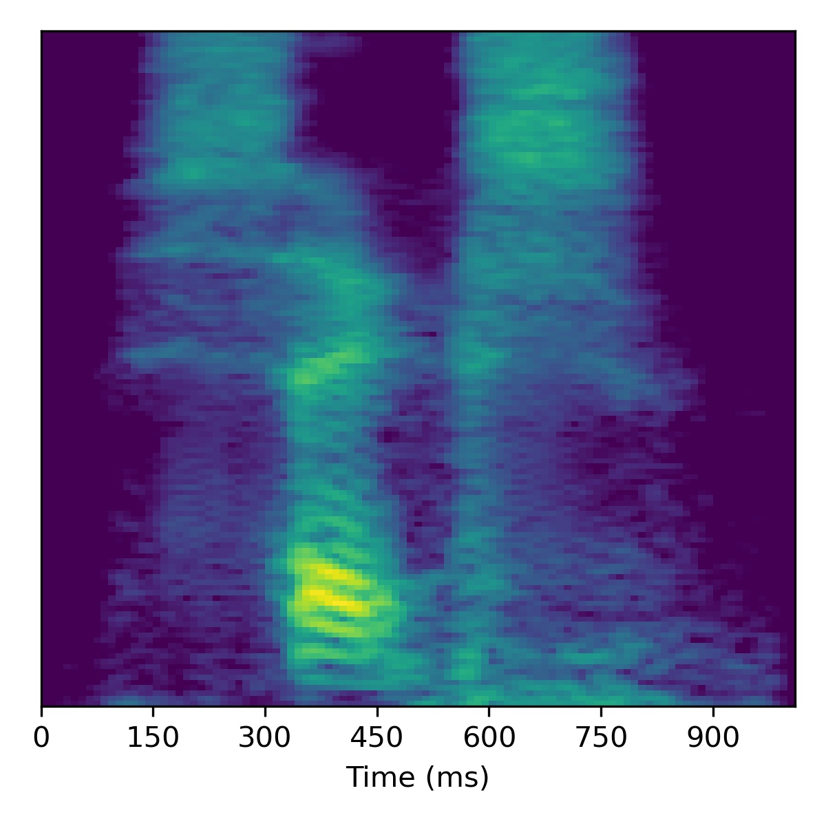
Unconditional samples
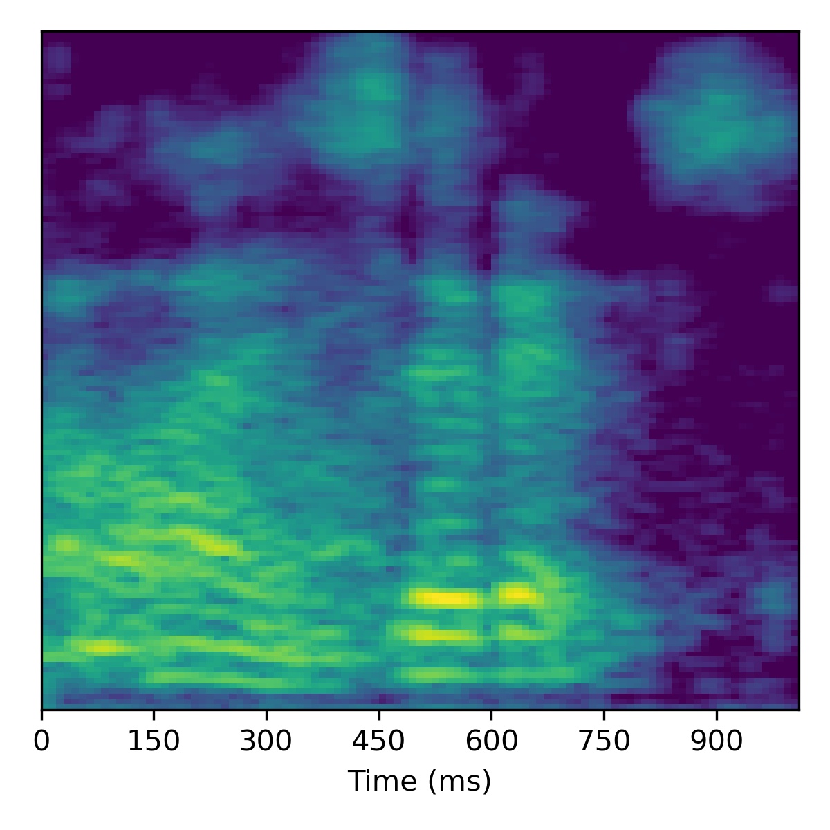
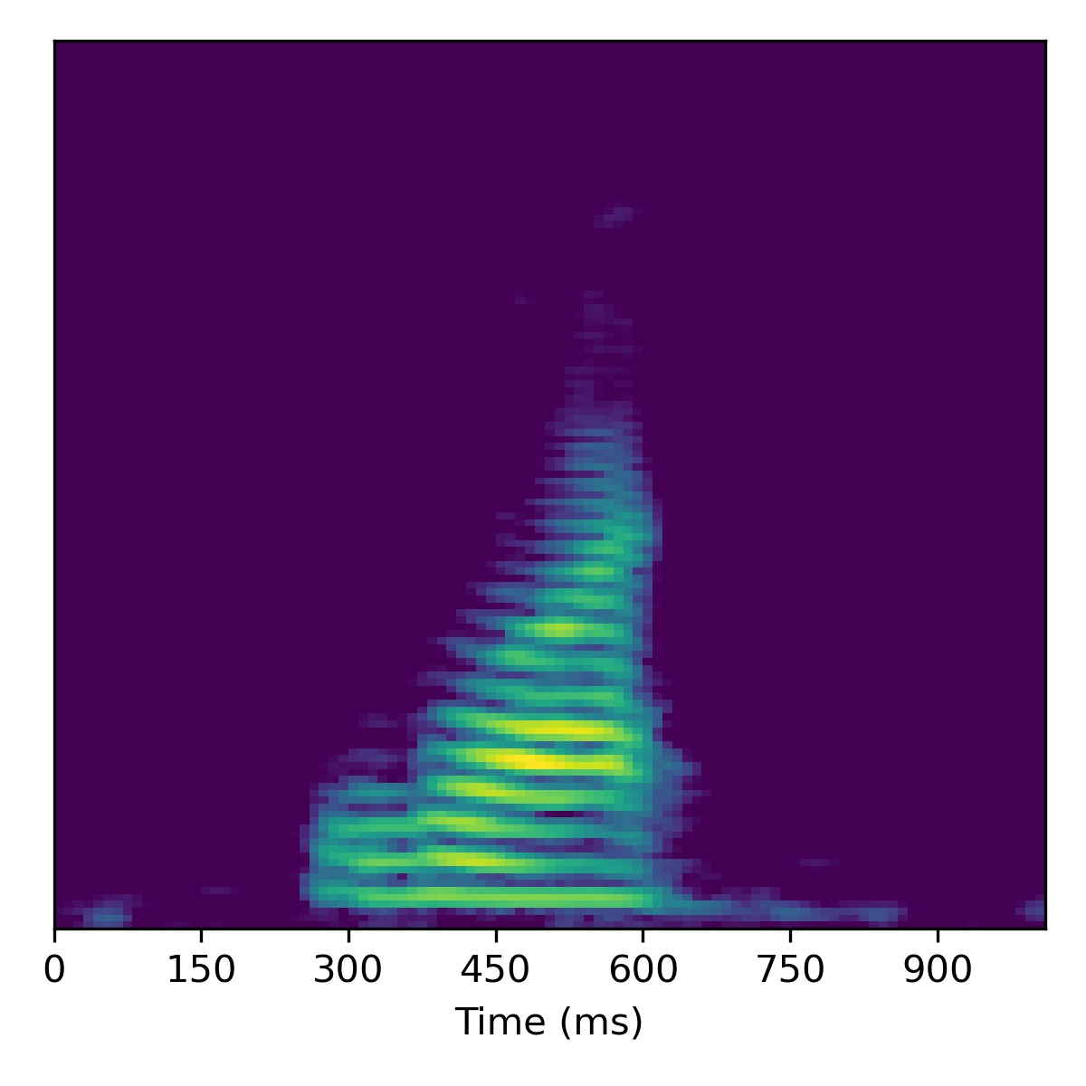
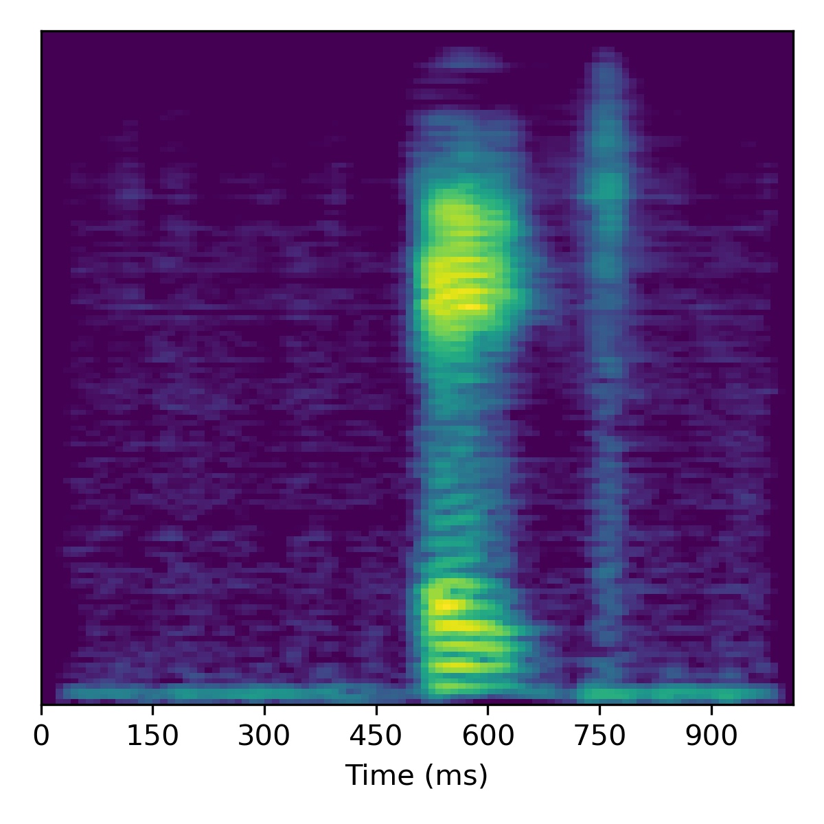
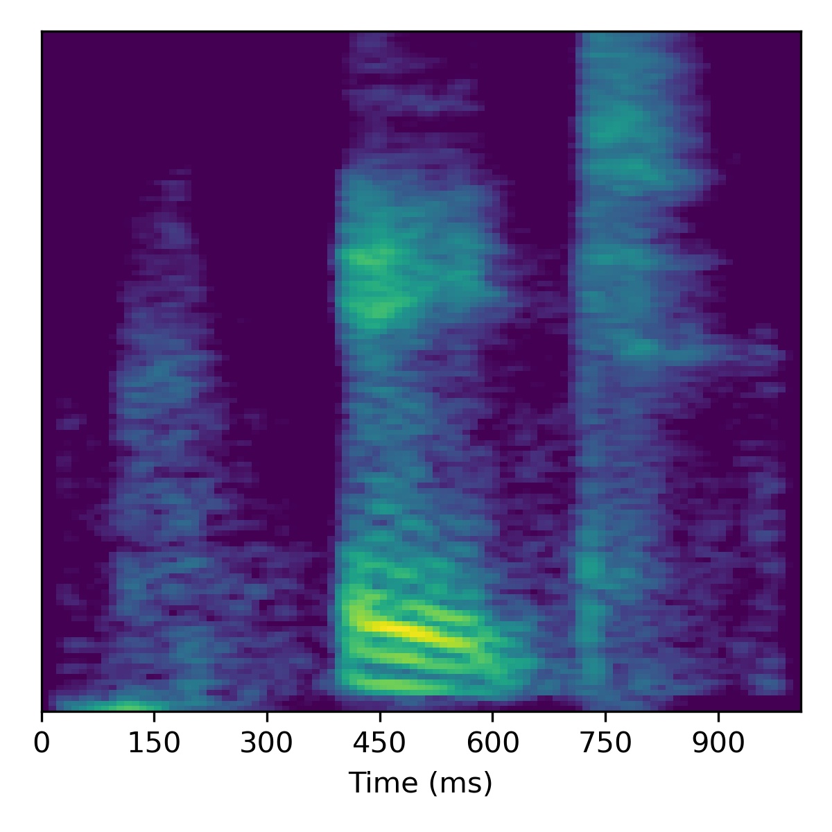
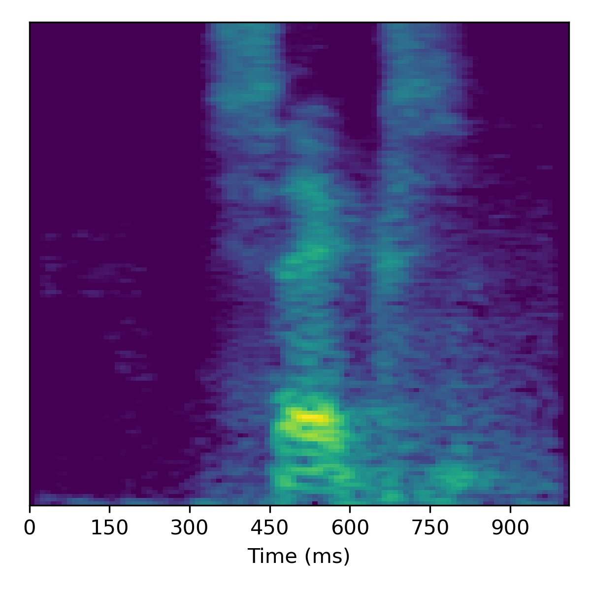
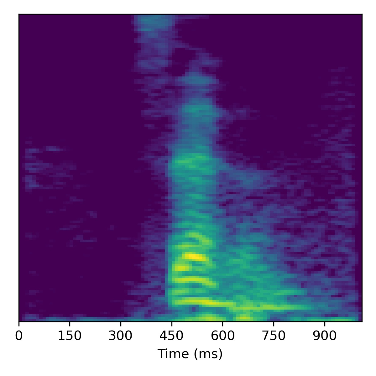
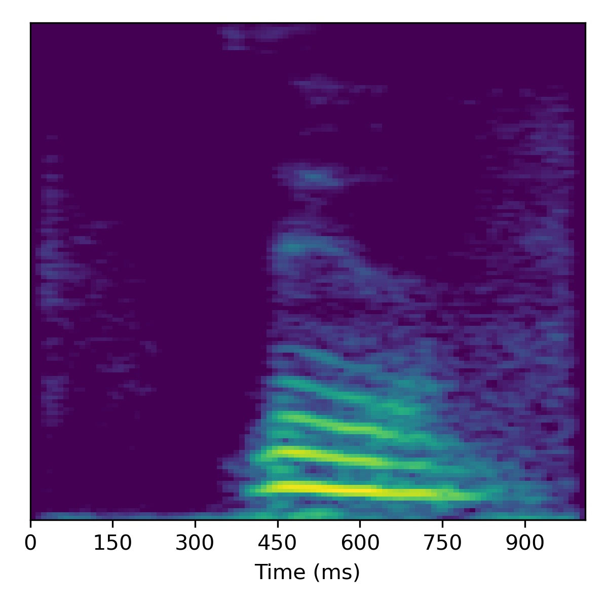
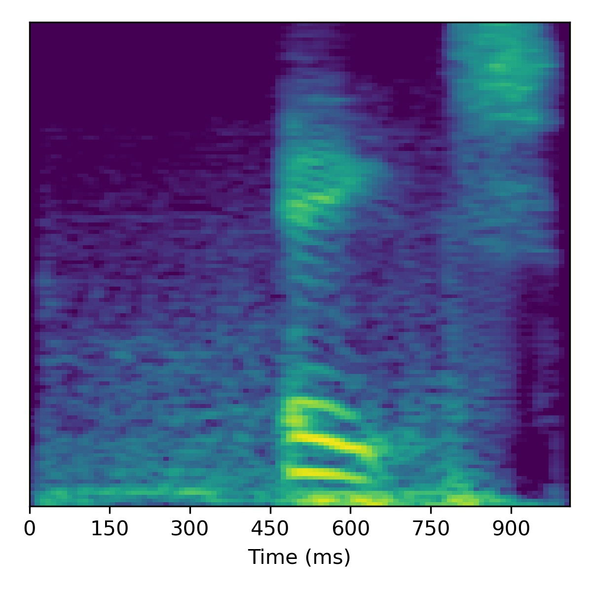
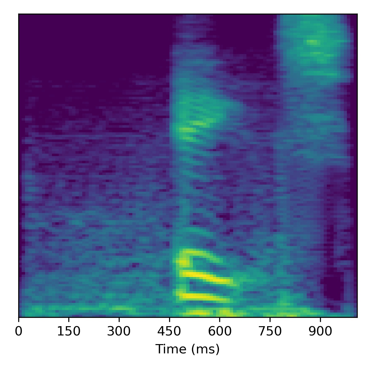
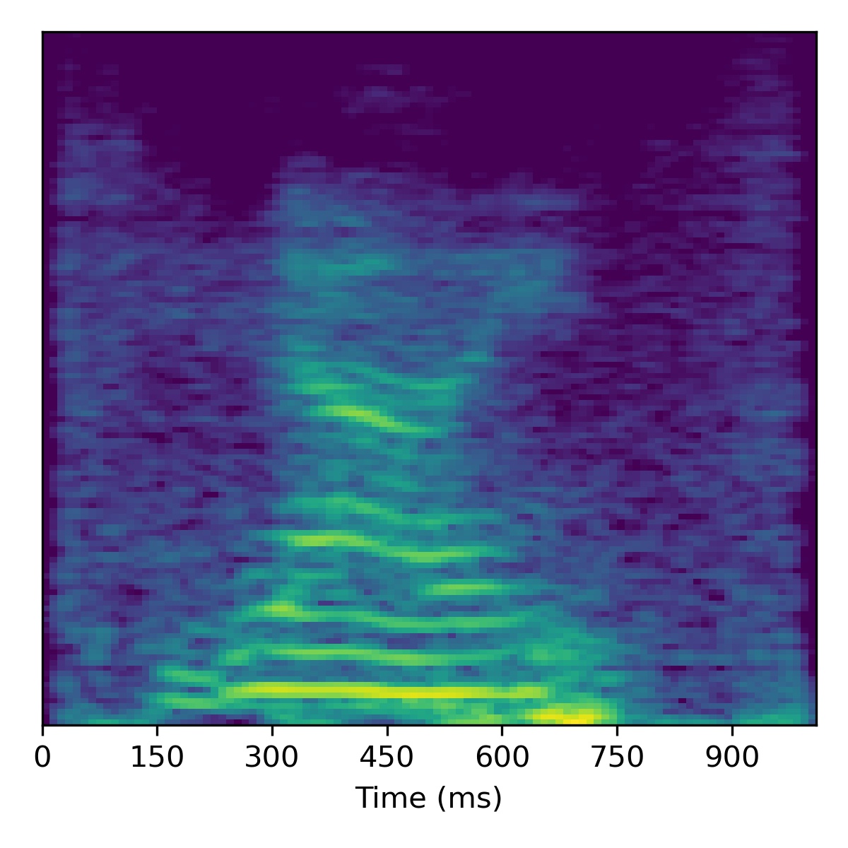
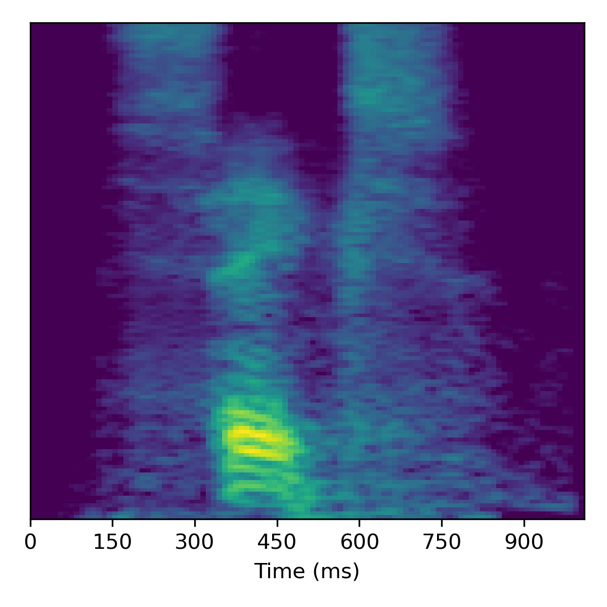
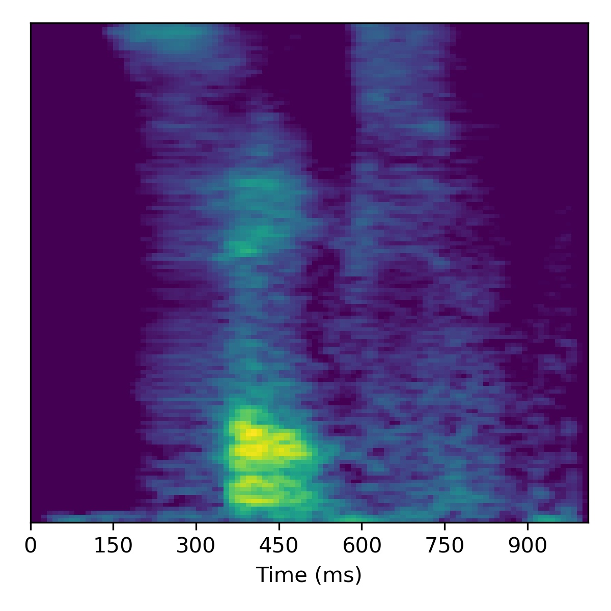
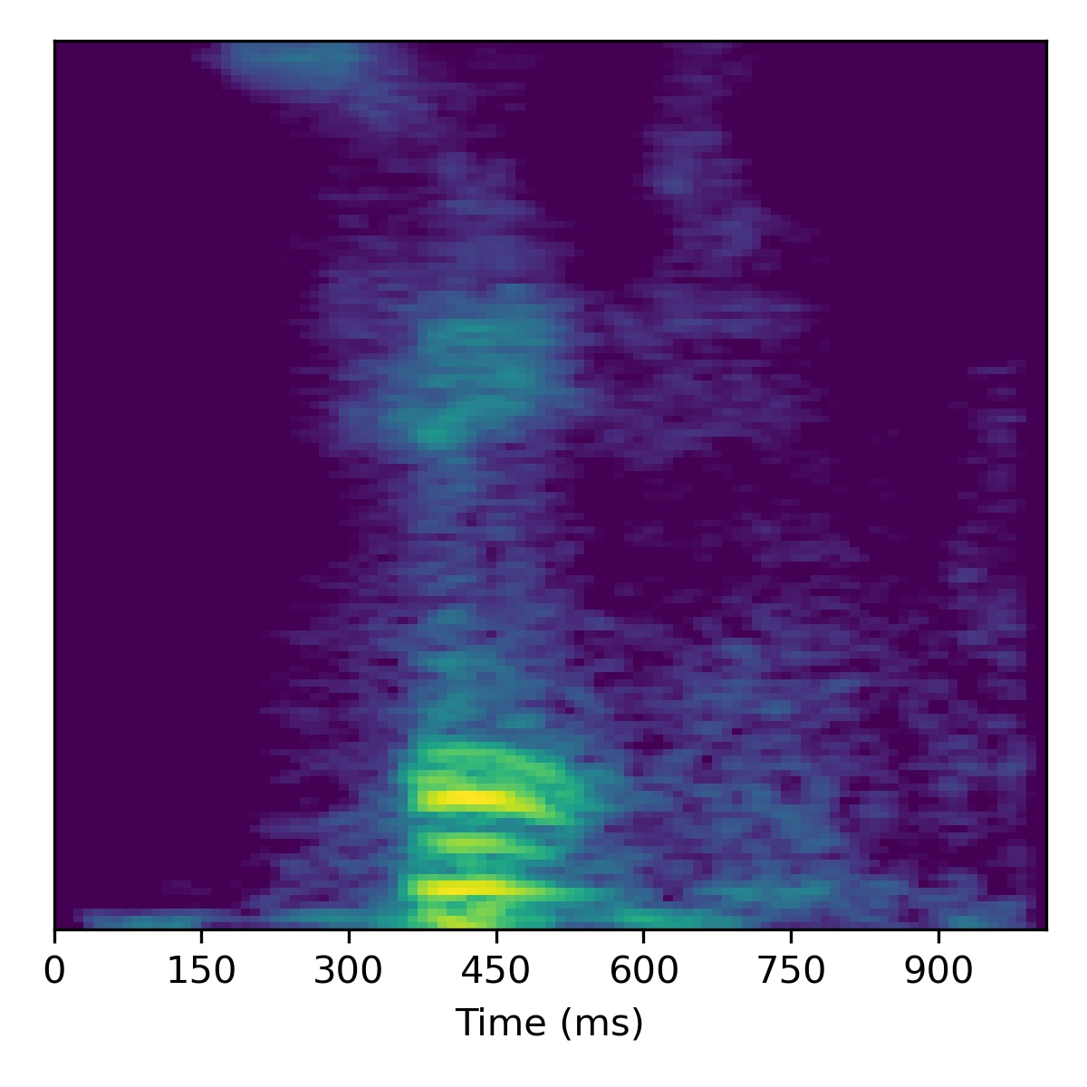
Below is a table of unconditional samples generated form each model using the same random seed (for torch, numpy, and base python):
| Sample | WaveGAN | SaShiMi | DiffWave | SaShiMi+DiffWave | ASGAN (mel-spec ver.) | ASGAN (HuBERT ver.) |
|---|---|---|---|---|---|---|
| 00 | 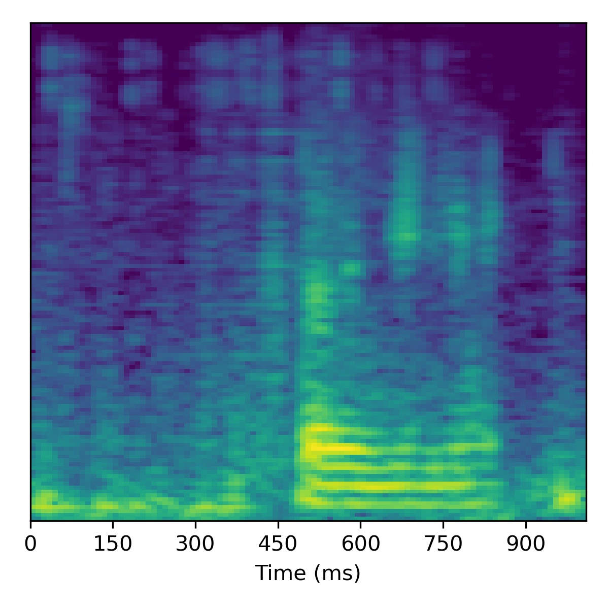 |
 |
 |
 |
 |
 |
| 01 | 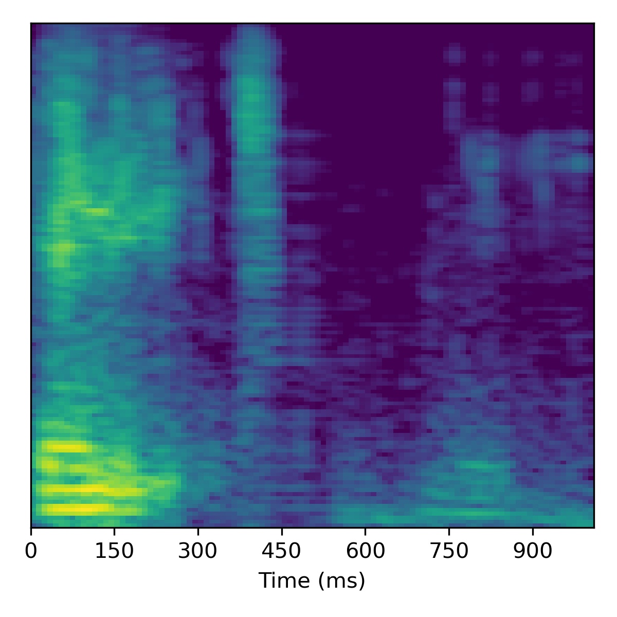 |
 |
 |
 |
 |
 |
| 02 | 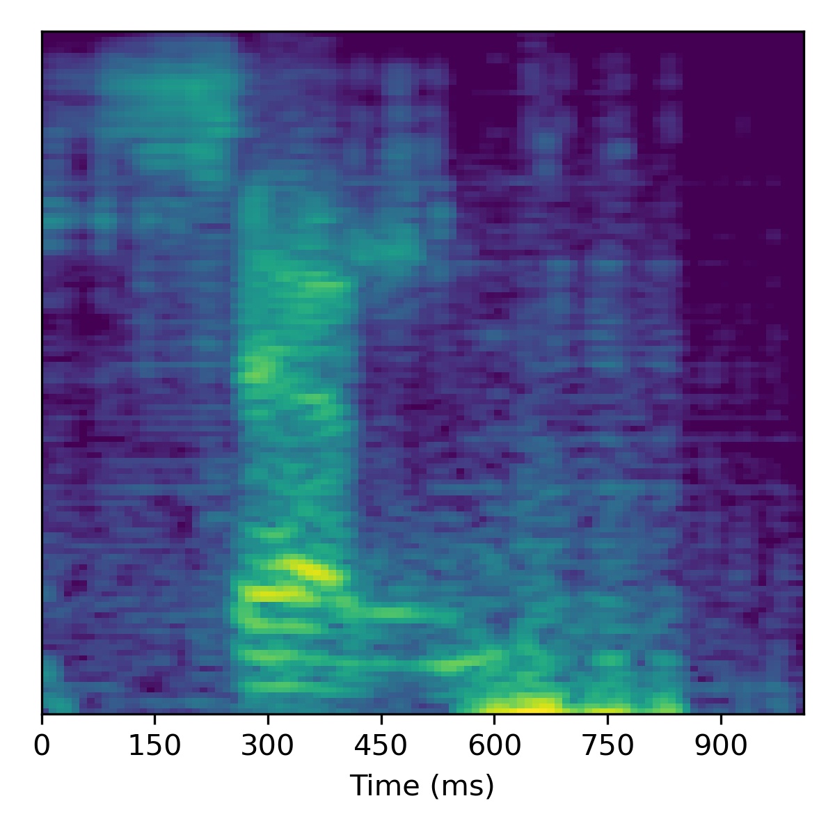 |
 |
 |
 |
 |
 |
| 03 | 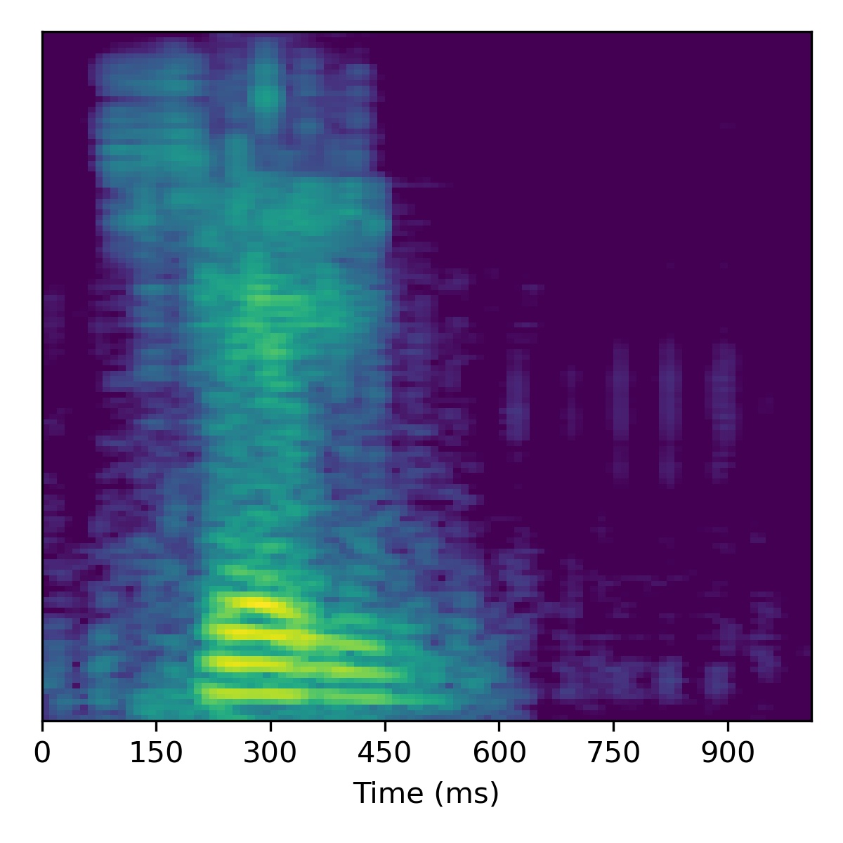 |
 |
 |
 |
 |
 |
| 04 | 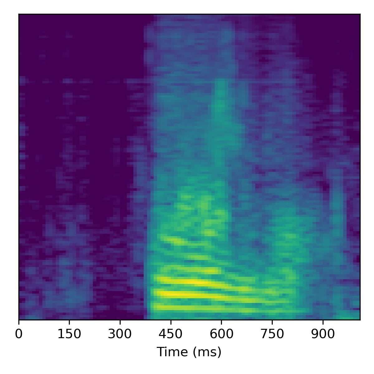 |
 |
 |
 |
 |
 |
| 05 | 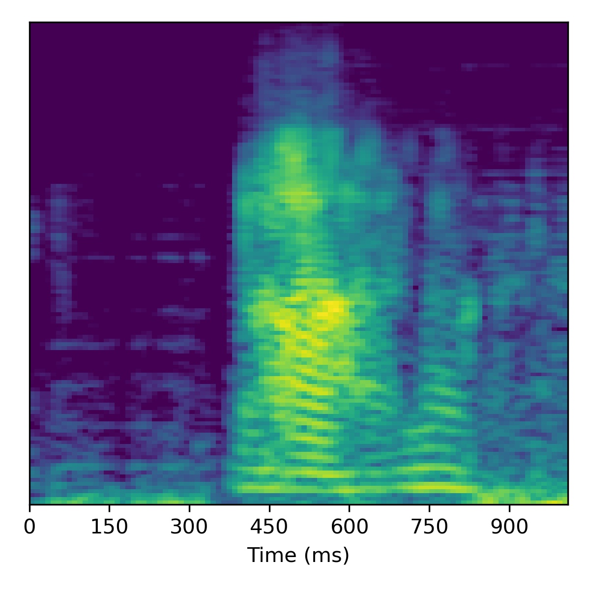 |
 |
 |
 |
 |
 |
| 06 | 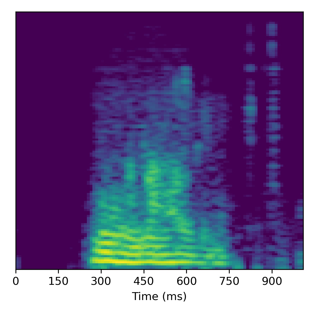 |
 |
 |
 |
 |
 |
| 07 | 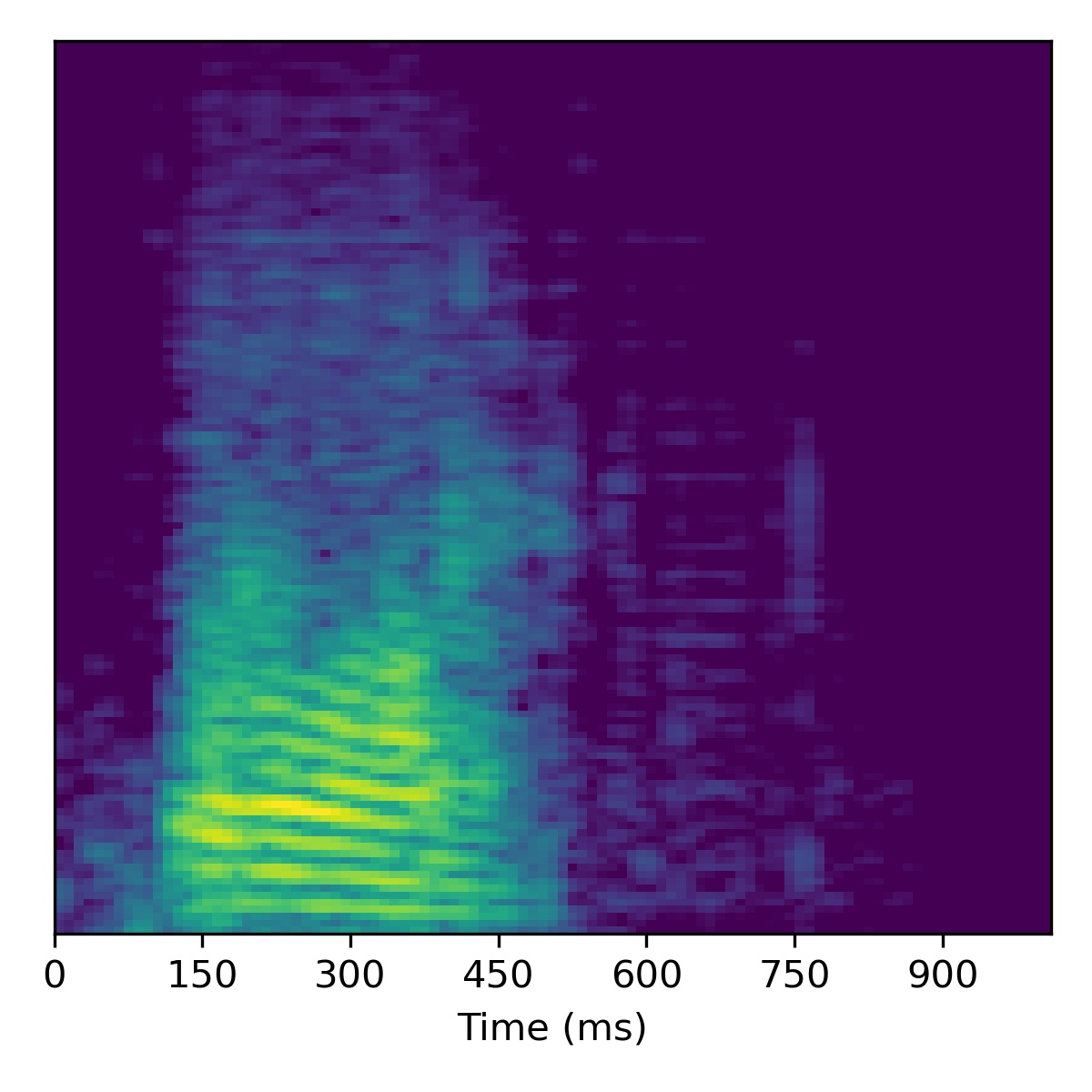 |
 |
 |
 |
 |
 |
| 08 | 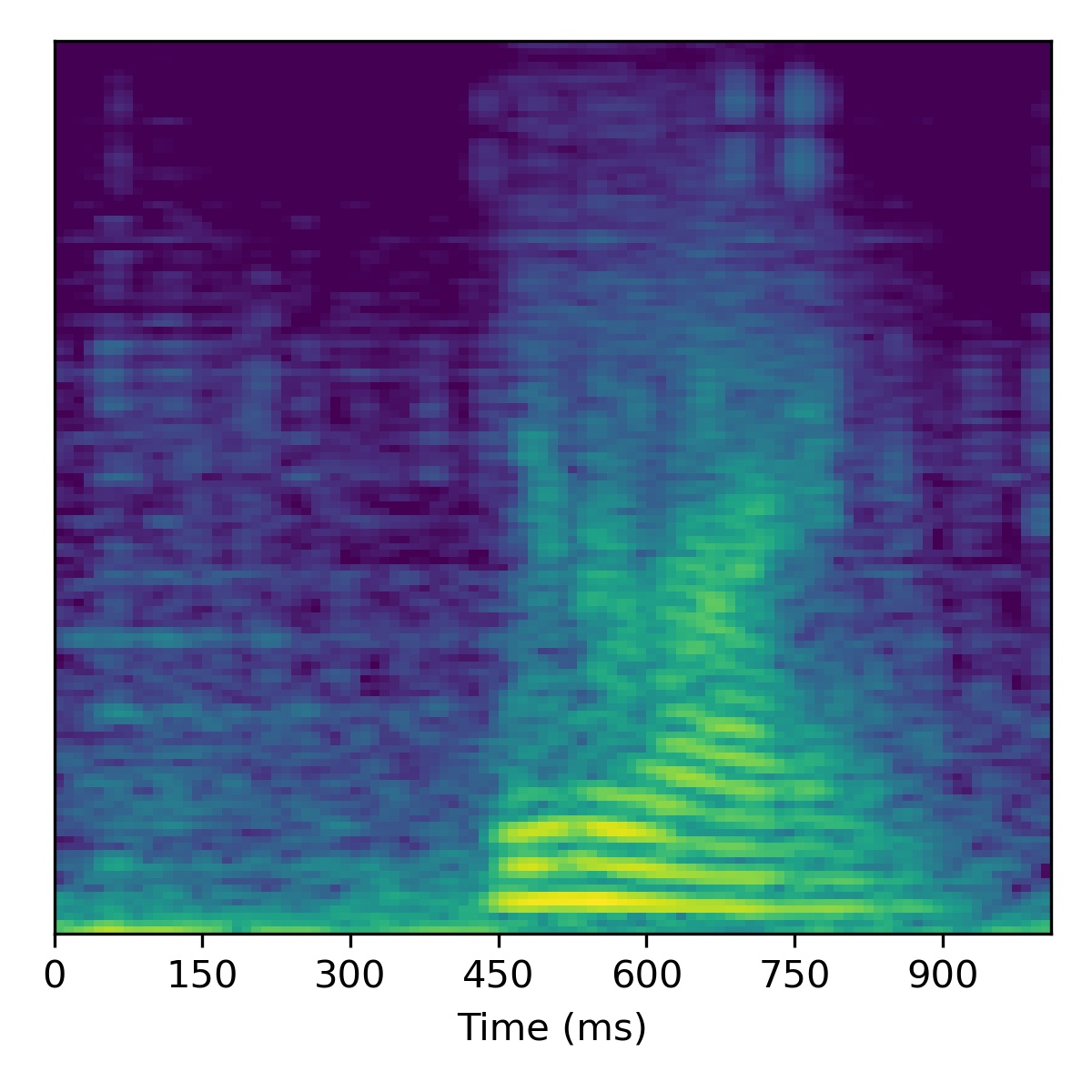 |
 |
 |
 |
 |
 |
| 09 | 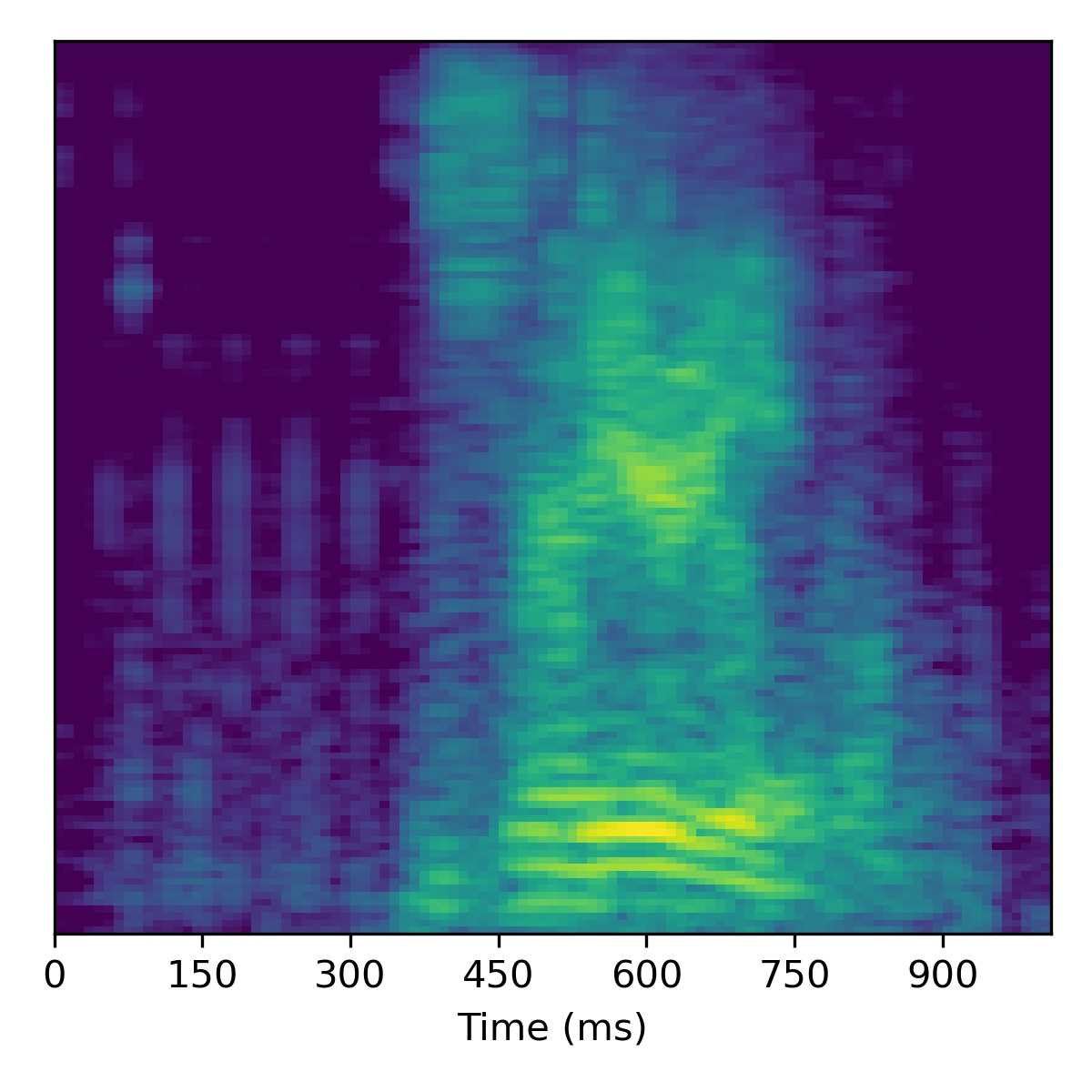 |
 |
 |
 |
 |
 |
Unseen tasks
In the following, we show a few examples of using ASGAN on unseen tasks.
To reiterate as in the paper, we define the course styles as those \(\mathbf{w}\) which are fed as input to the first 10 layers (first two Style Block groups) and the input to the base Fourier Feature layer.
The fine styles are those \(\mathbf{w}\) which are used as inputs to the last 5 modulated convolution layers (last two Style Block groups).
Voice conversion
To perform voice conversion from a speech feature sequence \(X_1\) to a speaker from another utterance’s features \(X_2\), start with the projection of \(X_1\) (i.e. \(\mathbf{w}_1\)) and then interpolate the fine styles between \(\mathbf{w}_1\) and \(\mathbf{w}_2\) to gradually change the speaker identity.
Several examples are given below (the first of which is the same example from the paper) using a truncation \(\psi=0.3\):
| Sample | Projected \(X_1\) | Projected \(X_2\) | Course styles: \(\mathbf{w}_1\) Fine styles: \(\mathbf{w}_1 + 0.5(\mathbf{w}_2 - \mathbf{w}_1)\) |
Course styles: \(\mathbf{w}_1\) Fine styles: \(\mathbf{w}_1 + 1.0(\mathbf{w}_2 - \mathbf{w}_1)\) |
Course styles: \(\mathbf{w}_1\) Fine styles: \(\mathbf{w}_1 + 1.5(\mathbf{w}_2 - \mathbf{w}_1)\) |
Course styles: \(\mathbf{w}_1\) Fine styles: \(\mathbf{w}_1 + 2.0(\mathbf{w}_2 - \mathbf{w}_1)\) |
|---|---|---|---|---|---|---|
| 00 | 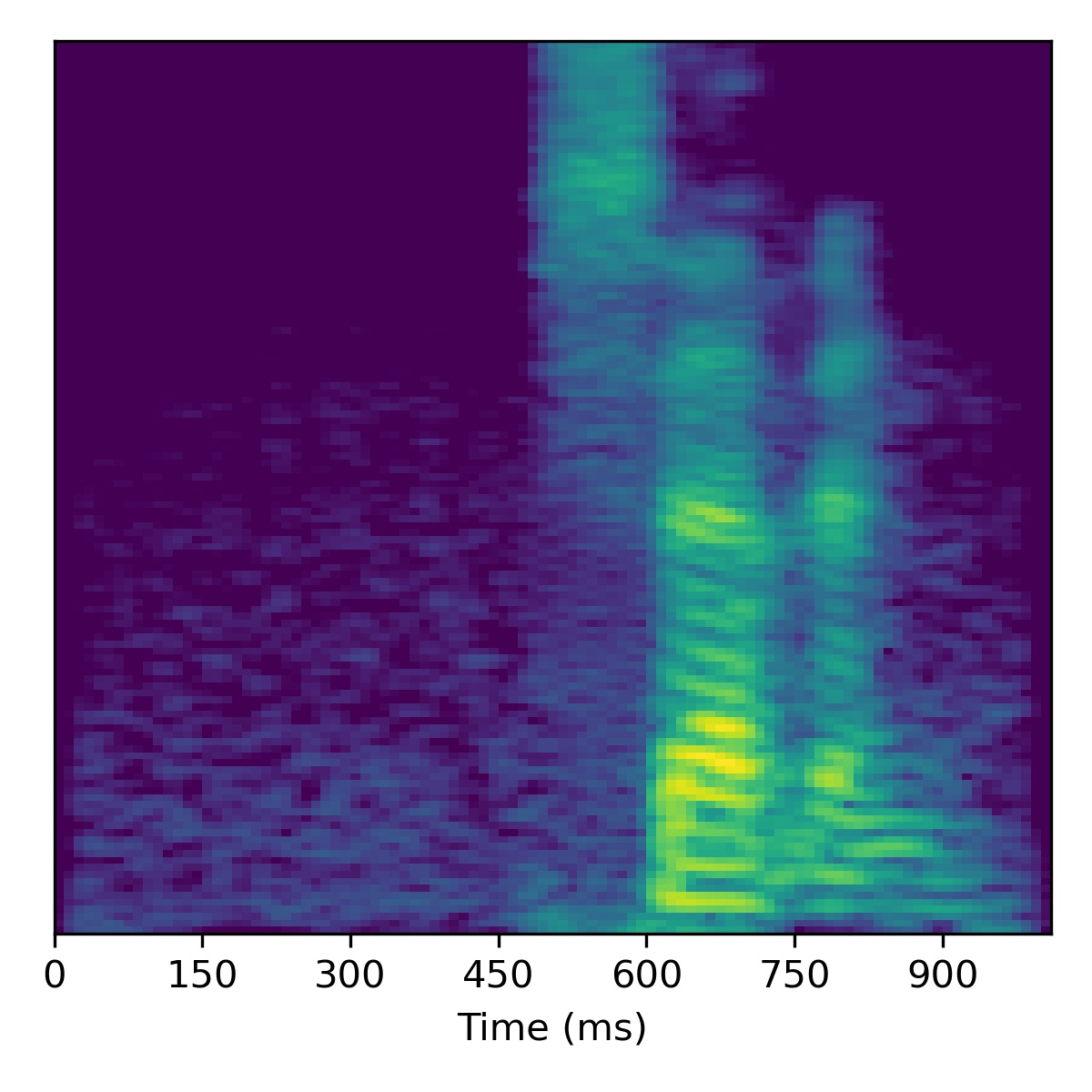 |
 |
 |
 |
 |
 |
| 01 | 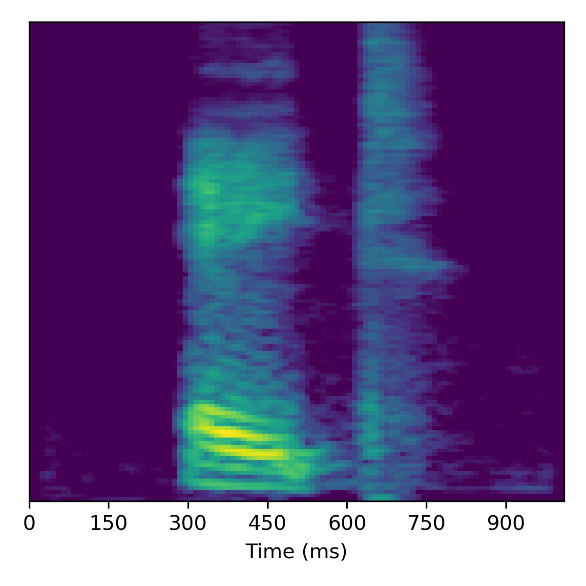 |
 |
 |
 |
 |
 |
| 02 | 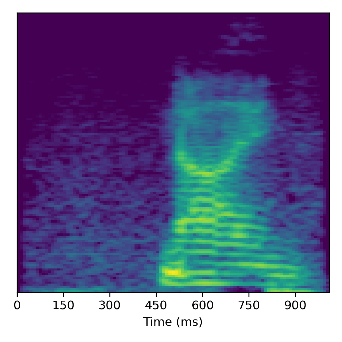 |
 |
 |
 |
 |
 |
| 03 |  |
 |
 |
 |
 |
 |
| 04 | 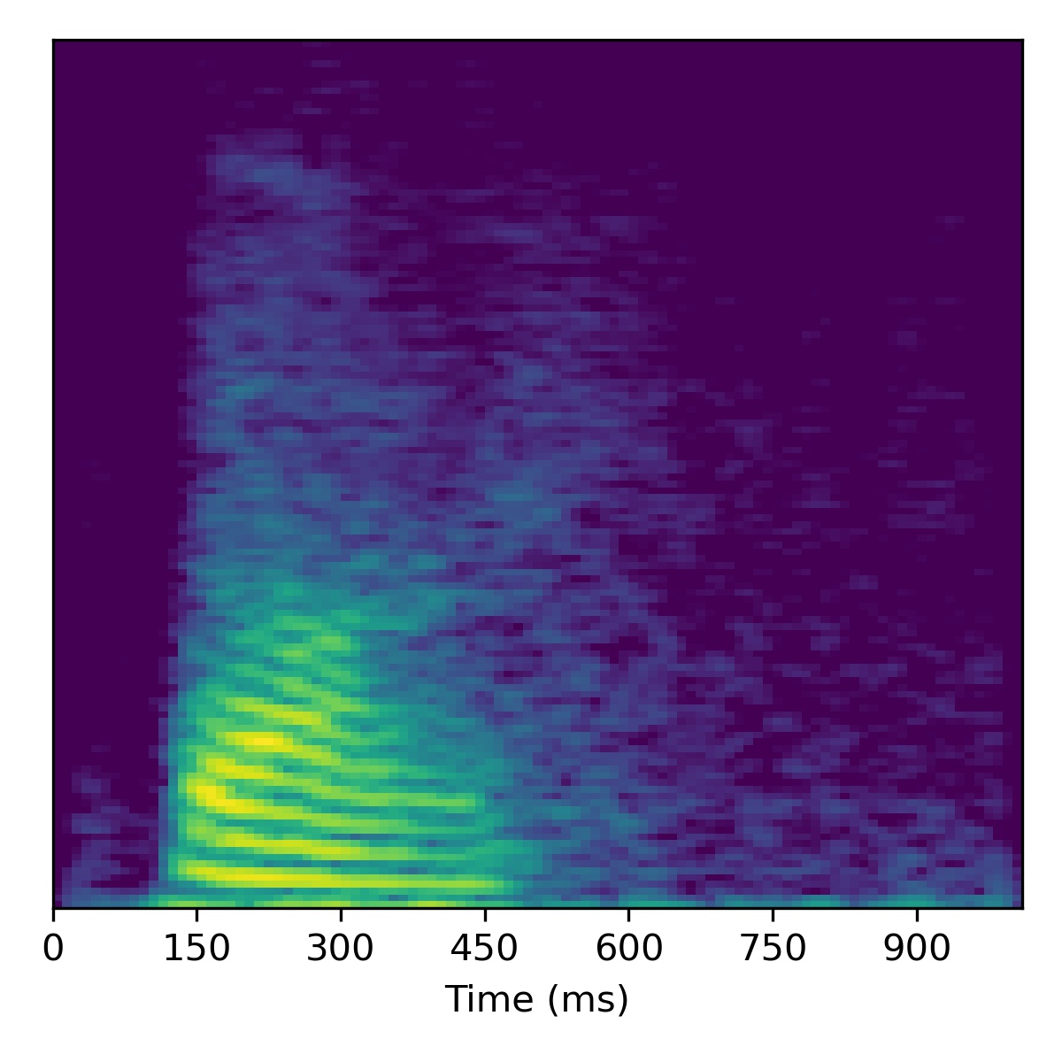 |
 |
 |
 |
 |
 |
| 05 |  |
 |
 |
 |
 |
 |
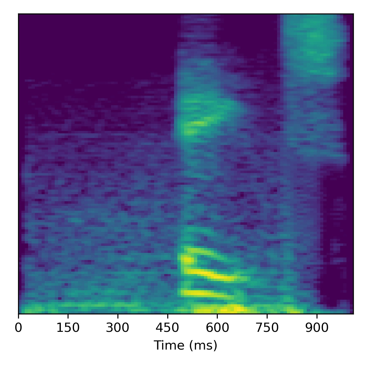
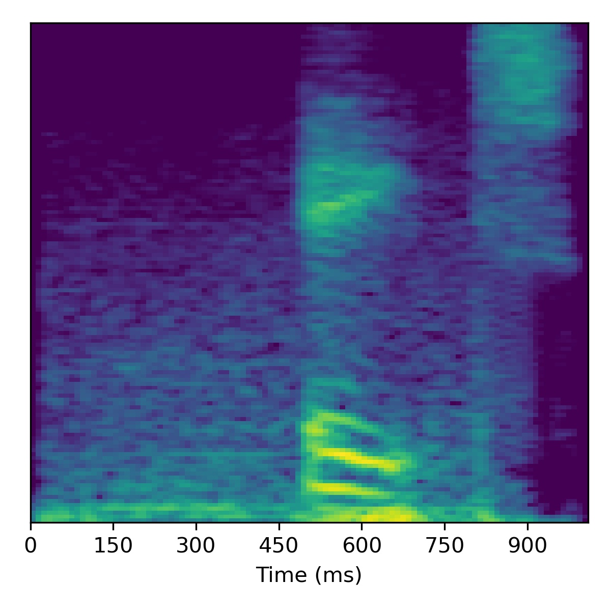
Digit conversion
To perform digit conversion (i.e. speech editing the transcript) from a speech feature sequence \(X_1\) to the digit spoken in another utterance’s features \(X_2\), we start with the projection of \(X_1\) (i.e. \(\mathbf{w}_1\)) and then interpolate the course styles between \(\mathbf{w}_1\) and \(\mathbf{w}_2\) to gradually change the speaker identity.
Several examples are given below (the first of which is the same example from the paper) using a truncation \(\psi=0.3\):
| Sample | Projected \(X_1\) | Projected \(X_2\) | Course styles: \(\mathbf{w}_1 + 0.5(\mathbf{w}_2 - \mathbf{w}_1)\) Fine styles: \(\mathbf{w}_1\) |
Course styles: \(\mathbf{w}_1 + 0.8(\mathbf{w}_2 - \mathbf{w}_1)\) Fine styles: \(\mathbf{w}_1\) |
Course styles: \(\mathbf{w}_1 + 1.5(\mathbf{w}_2 - \mathbf{w}_1)\) Fine styles: \(\mathbf{w}_1\) |
Course styles: \(\mathbf{w}_1 + 2.0(\mathbf{w}_2 - \mathbf{w}_1)\) Fine styles: \(\mathbf{w}_1\) |
|---|---|---|---|---|---|---|
| 00 | 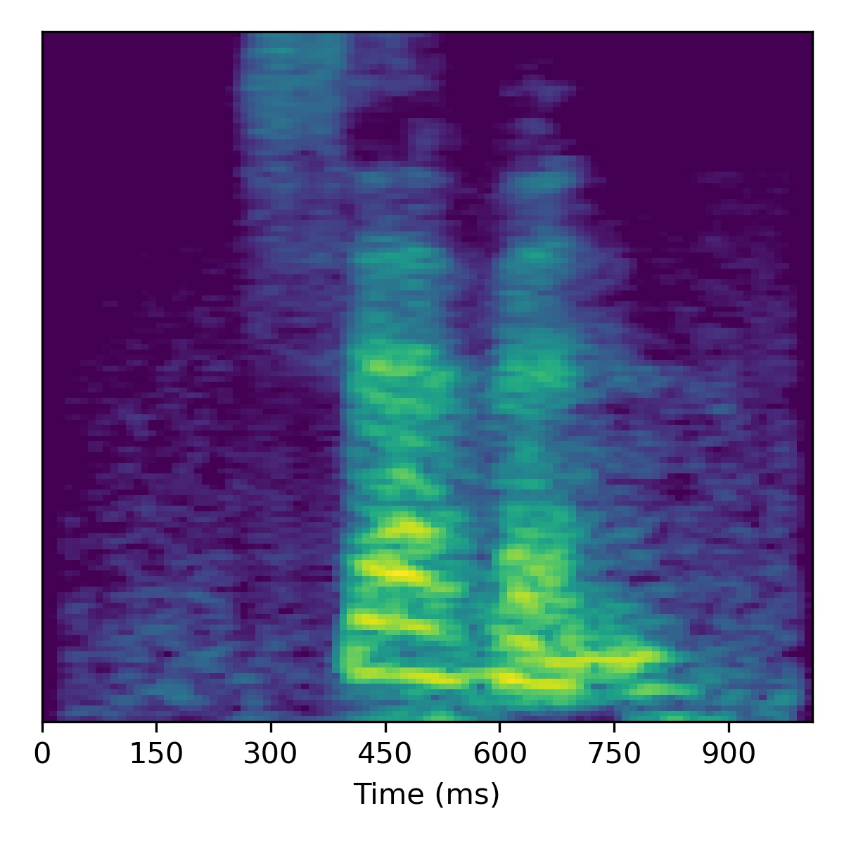 |
 |
 |
 |
 |
 |
| 01 |  |
 |
 |
 |
 |
 |
| 02 |  |
 |
 |
 |
 |
 |
| 03 | 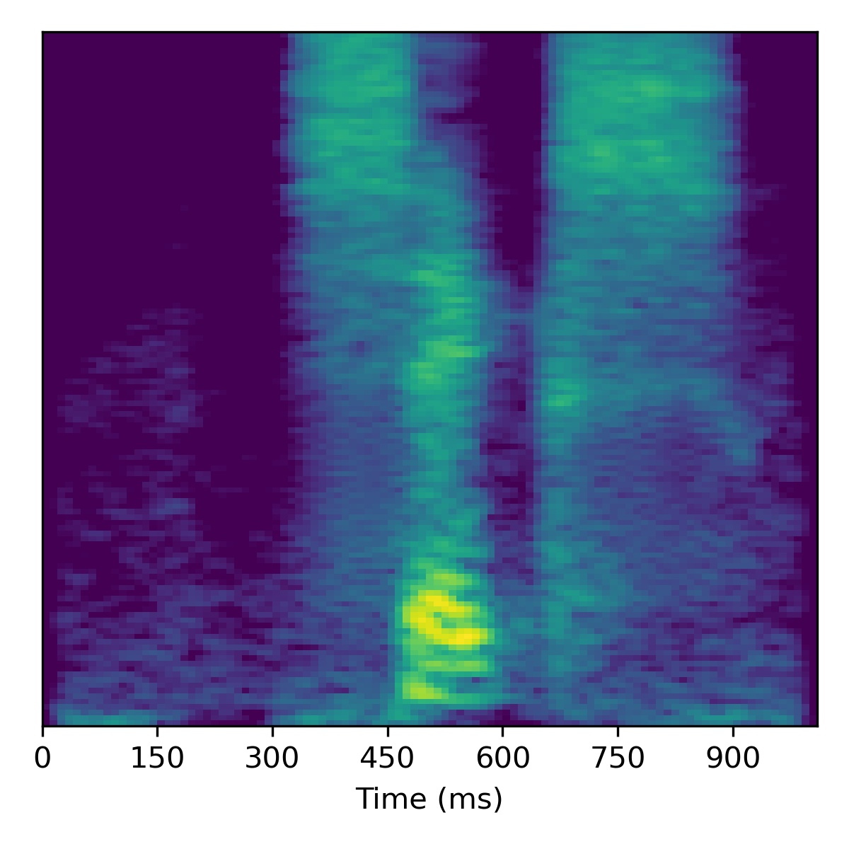 |
 |
 |
 |
 |
 |
| 04 |  |
 |
 |
 |
 |
 |
| 05 | 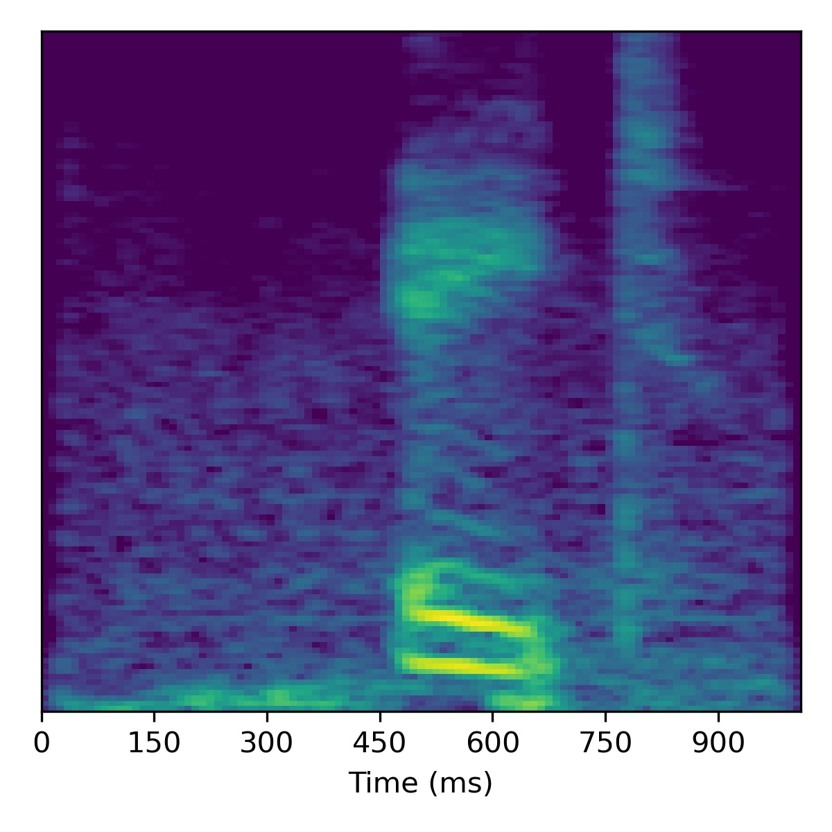 |
 |
 |
 |
 |
 |
Speech enhancement
For speech enhancement we follow the procedure outlined in the paper, using \(N=10\) and \(\sigma^2=0.001\). Concretely, after projection, we move in the direction of the decreasing noise vector \(\mathbf{\delta}\) (or in the opposite direction to increase noise).
Several examples are given below (the first of which is the same as in the paper), where all the samples in the left column are particularly noisy utterances found in the SC09 test set:
| Sample | Raw \(X_0\) | Projection \(\tilde{X}_0\) | All styles: \(\mathbf{w}_0 -3 \mathbf{\delta}\) | All styles: \(\mathbf{w}_0 + 3\mathbf{\delta}\) | All styles: \(\mathbf{w}_0 + 6\mathbf{\delta}\) | All styles: \(\mathbf{w}_0 + 9.0\mathbf{\delta}\) |
|---|---|---|---|---|---|---|
| 00 | 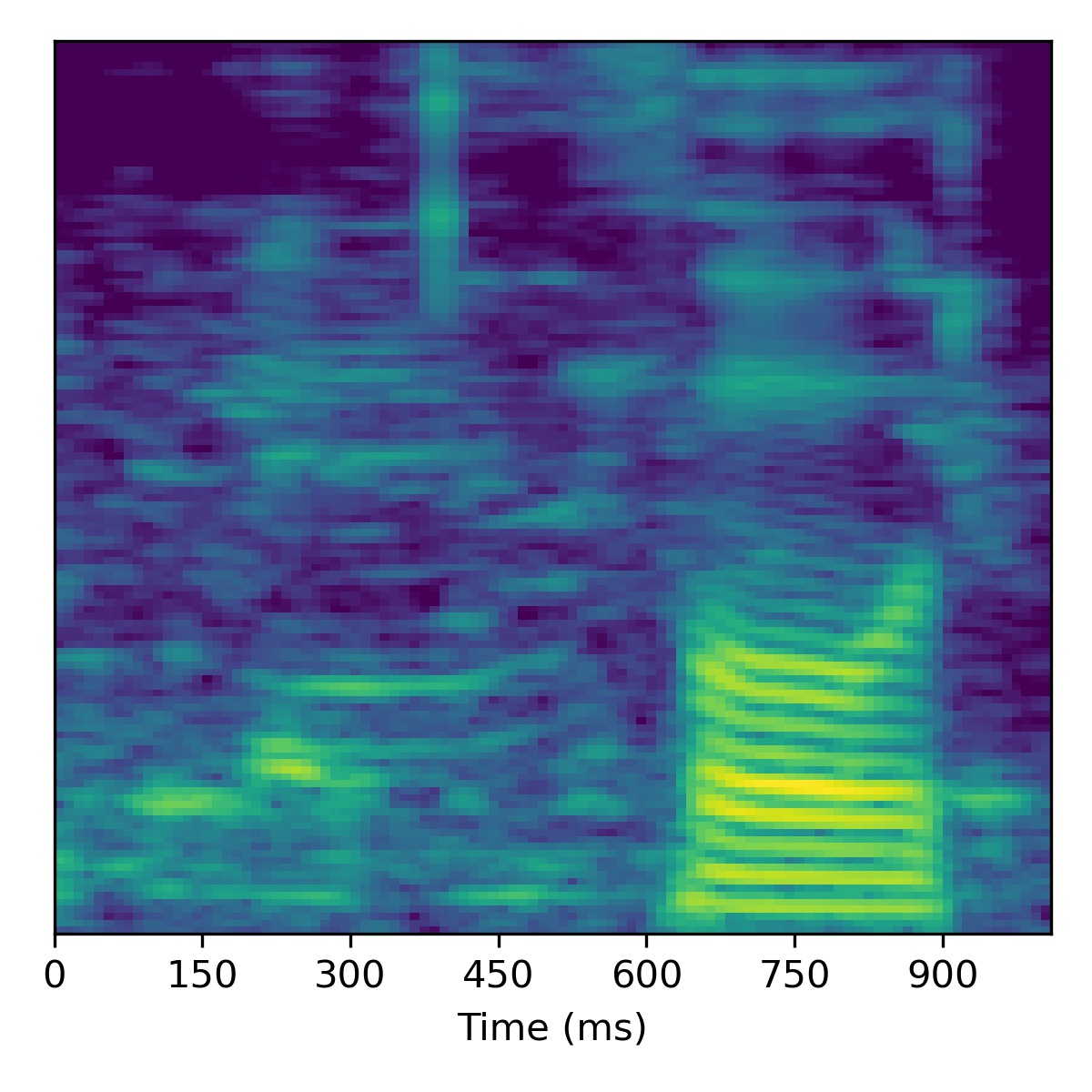 |
 |
 |
 |
 |
 |
| 01 | 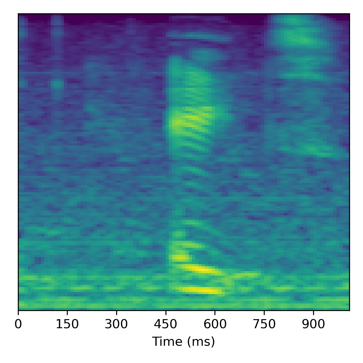 |
 |
 |
 |
 |
 |
| 02 | 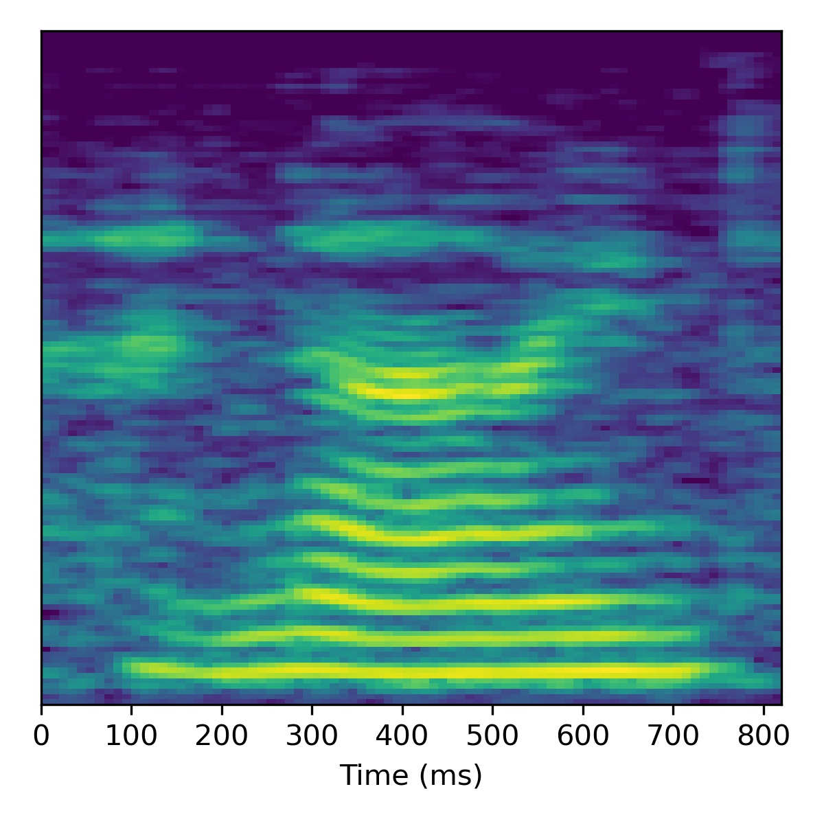 |
 |
 |
 |
 |
 |
| 03 | 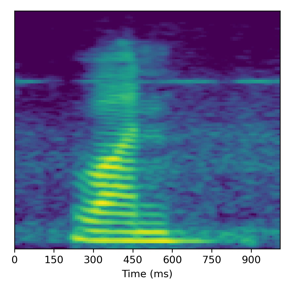 |
 |
 |
 |
 |
 |
| 04 | 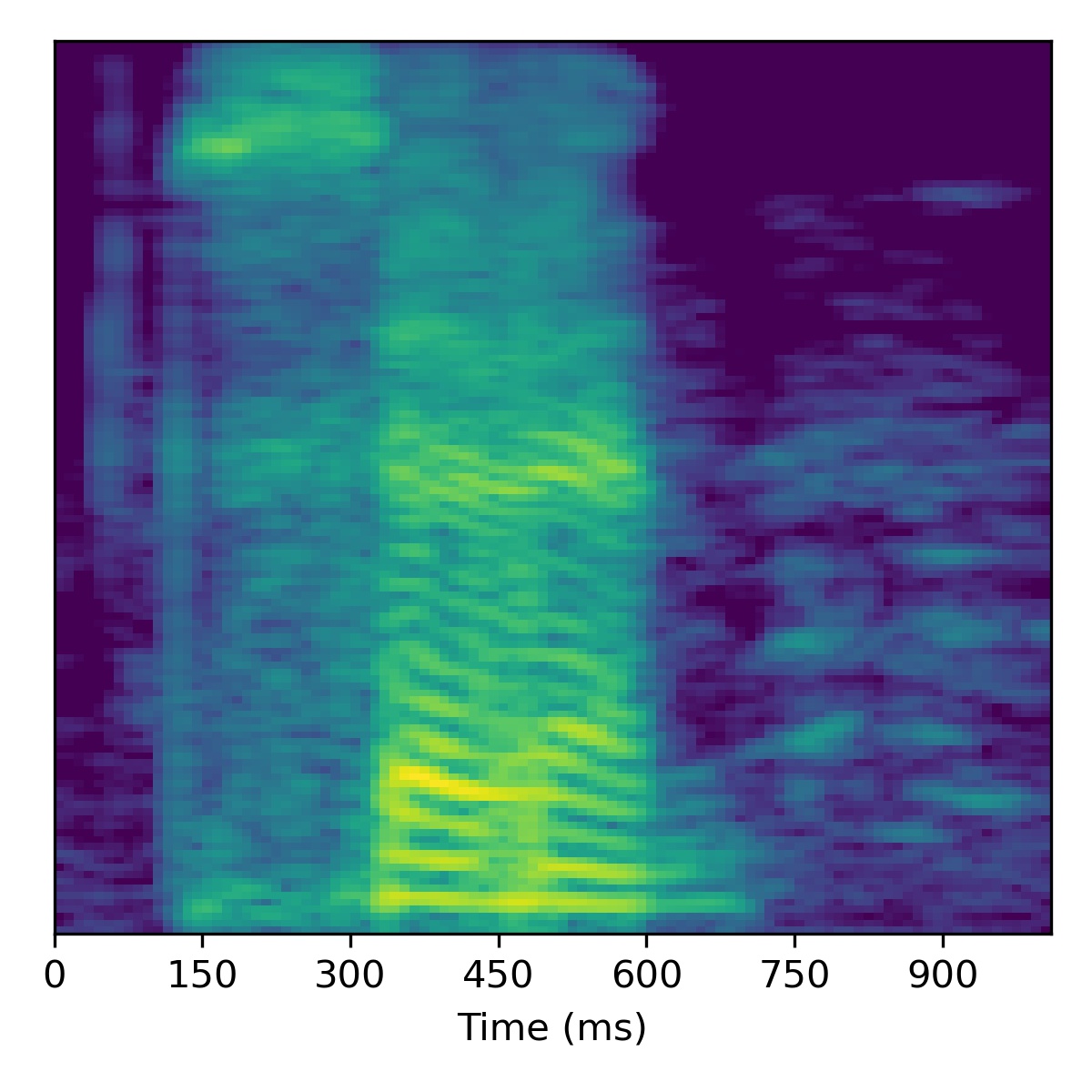 |
 |
 |
 |
 |
 |
| 05 |  |
 |
 |
 |
 |
 |
Bonus
Bonus 1: Out of domain sample
As a bonus, here is what happens when attempting to project a extreme out-of-domain sample – one of the authors saying the “SLT” (a word/acronym not even remotely similar to the dataset)! After projection, we try to apply voice conversion to this extreme out of domain sample \(X_1\). To get this to work, we had to modify the inversion technique by using 3000 updates instead of 1000.
| Original waveform \(X_1\) |
Projected \(X_1\) | Projected \(X_2\) | Course styles: \(\mathbf{w}_1\) Fine styles: \(\mathbf{w}_1 + 0.5(\mathbf{w}_2 - \mathbf{w}_1)\) |
Course styles: \(\mathbf{w}_1\) Fine styles: \(\mathbf{w}_1 + 1.0(\mathbf{w}_2 - \mathbf{w}_1)\) |
Course styles: \(\mathbf{w}_1\) Fine styles: \(\mathbf{w}_1 + 1.5(\mathbf{w}_2 - \mathbf{w}_1)\) |
Course styles: \(\mathbf{w}_1\) Fine styles: \(\mathbf{w}_1 + 2.0(\mathbf{w}_2 - \mathbf{w}_1)\) |
|---|---|---|---|---|---|---|
 |
 |
 |
 |
 |
 |
 |
As we can see, it doesn’t perform voice conversion very well! We suspect this is because the projected point \(\mathbf{w}_1\) is so far out-of-domain that it lies far away from the manifold upon which the training data lies within the \(W\)-space. Intuitively, we hypothesize that because \(\mathbf{w}_1\) is so far out of domain, the part of the \(W\)-space it inhabits is no longer linearly disentangled as it is so far away from the other points. Since things are no longer linearly disentangled, linear operations we perform to try and achieve voice conversion fail in strange ways, as seen above.
Bonus 2: Latent interpolation videos
To give a final visual indication of the disentanglement of the latent space, we perform a walk within the latent space between several sampled \(\mathbf{w}\) vectors to produce a video similar to those typically shown for unconditional image synthesis models. For the videos below we use a truncation \(\psi=0.5\) and linearly interpolate within the \(W\)-space between several anchor points:
| Example 1 | Example 2 | Example 3 |
|---|---|---|
Citation
Please find our bibtex citation:
@inproceedings{baas2022asgan,
  title={{GAN} you hear me? Reclaiming unconditional speech synthesis from diffusion models},
  author={Baas, Matthew and Kamper, Herman},
  booktitle={IEEE SLT Workshop},
  year=2022
}
Thank you for checking out our work!