Using Fastai v2 to approximate electric fields for dipole antenna arrays

by Matthew Baas

Using UNets to estimate H-plane electric field magnitudes of arbitrary dipole antenna arrays in real time.

TL;DR: After learning some basic antenna theory, and noting how long most simulation packages like FEKO or the CST suite take to calculate electric/magnetic fields for even simple antenna arrays, I wanted to see if one can train a neural network to get a good first-approximation of the fields for any arbitrary antenna array in a fraction of the time (ideally constant for a given volume of interest). But, that problem is quite broad and will require much work and careful thought. So first I decided to see if it was even reasonable to expect a neural network to infer electric field patterns given current source distributions. That is what I explore here.

Background

Electromagnetic field patterns of arbitrary current source distributions are usually too complex to find a closed-form solution by hand, and they are usually solved with simulation software either in the time domain or the frequency domain. Packages like FEKO, CST suite, and MEEP all offer various ways of doing this. All these methods, however, can take a fair amount of time for any moderately complicated current source geometry.

So, here I try to apply deep learning using UNets to see if one can speed this simulation up (for a first approximation, at least). If one can speed up the simulation to faster than real time, then it opens the door to more interesting downstream tasks like inferring current source distributions to generate a particular near-field pattern, or even trying to combine style transfer with it to get one antenna structure to (by adjusting phases/magnitudes) have the same radiation pattern as another antenna geometry…

The goal, concretely

The end problem of simulating all 3D electric/magnetic fields of arbitrary current source distributions, materials, and geometries is hectically complex and a bit above my current resources and capabilities. So first, to see if aiming for such a goal is even realistic, I first try to see if a simpler, constrained proof-of-concept is nicely solvable.

For this proof-of-concept, the goal is to predict the magnitude of the z-component of the full electric field intensity in the H-plane of constrained arbitrary antenna arrays. To do this, I used supervised learning whereby I generated many (1000) simulations of arbitrary antenna arrays and their associated electric fields, and then trained a Unet to take the current source distributions as input and produce the resulting electric field magnitude as output.

Simplifying constraints

For each simulation of an arbitrary antenna array, the following constraints are set. For each antenna array:

• All antenna elements are hertzian dipoles.
• All antenna elements are in phase.
• All antenna elements radiate at the same fixed frequency of 200GHz.
• Each dipole is aligned with the z-axis (the dipole, and its current is z-directed), and each dipole lies in the xy plane.
• The magnitude of the (AC) current in each antenna element will be the same at 1mA.

The simulation will also have the constraints:

• The simulation will be bounded to a region near to the current sources. In particular, it will be a 10mm x 10mm region centered on the origin, and several antenna elements will be placed within this region.
• The simulation medium is a vacuum.
• The simulation will use the MEEP python package to simulate the z-component of the electric field in the H-plane (xy plane) of the antenna elements using its frequency domain solver.
  • The 10mm x 10mm simulation region will be surrounded by a 2mm thick border of a perfectly matched layer. This is mostly to satisfy MEEP, which needs boundary conditions. It is equivalent to saying that the vacuum medium continues in all directions indefinitely, and we only look at the fields in the 10mm x 10mm region centered on the origin.
  • The resolution of the simulation is 40px/mm. So with 10mm x 10mm, the produced matrix from MEEP for each simulation will be 400x400 px.

Each simulation will vary in the following ways:

• The number of antenna elements is chosen uniformly at random between 2 and 10.
• The location of each antenna element is chosen uniformly at random to be within a 9.5mm x 9.5mm square (centered on the 10mm x 10mm simulation cell).

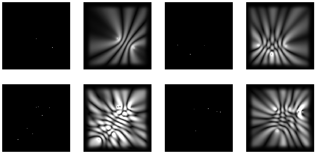
For visualization, below is the setup of one of these simulations where 3 antenna elements are chosen in the positions shown. Each simulation will have a setup similar to the below.

The simulation in MEEP produces the image imposed on the xy-plane (also the H-plane), whereby the brighter the color, the larger the magnitude of the z-component of the electric field at that point. Recall that since these are the total electric fields, at distances this close to each antenna element the near-field terms dominate, hence the pattern is somewhat complex compared to what we might expect in the far-field region.

Neural network setup

Since image-to-image neural networks are quite well developed in the literature, I use them and encode the current distributions and resulting electric fields as 2D images. Concretely, the neural network input and output are both images from the xy plane. The input image is a one-hot black-and-white image being white where a Hertzian dipole is located, and black otherwise. The output which the neural network needs to predict is the black-and-white image of \(|E_z|\), like the image imposed on the xy-plane in the previous diagram.

UNet setup: the details

• Use Fastai v2 (and a little Pytorch) libraries for training and data pipeline/transformation.
• Use Fastai v2’s implementation of unet_learner to construct the UNet architecture, with
  • a mean square error (MSE) loss function
  • an architecture built from a pretrained resnet18, resnet34, and resnet52 (see later on for results and comments when using the different architectures).
  • instance norm (and not batch norm).
• The data (input and output image) was transformed at test time by applying a random dihedral transform (left/right flip, up/down flip, any 90 degree rotation). This increases the diversity of input images the unet sees.
  • I opted to not use arbitrary rotations as well since the PML border kind of messed with it, and zooms could cause issues since the neural network doesn’t know what unit distance it is working with, which would make predicting arbitrary on images with changing zooms fail quite badly.
• The input one-hot current source images are cast to a 3x400x400 RGB image tensor to work with the existing unet architecture. The output is still a black-and-white 1x400x400 tensor representing the (normalized) \(|E_z|\) in the H-plane.

To visualize this a bit more, below is an example batch of 4 input images and their associated labels (as produced by MEEP). The MSE loss function aims to make the output of the UNet match the label as close as possible.

There is probably a more sophisticated way of doing this which would make it easier for the neural network, such as including channels with pixel values proportional to \(\frac{1}{r}\) or channels for the phase of each source, or any number of other extensions. But for a first attempt, this is simple, fairly general, and makes integration with an existing UNet architecture very very clean. For this experiment I generated 1000 images, 800 for training and 200 for validation.

The code: Fastai v2

Fastai is a great library for prototyping neural net stuff, particularly for vision applications. A few of my previous projects have used it and it works quite nicely and is fairly intuitive. Now, the authors of fastai (Jeremy Howard and Sylvain Gugger mainly) are developing a rewrite successor called fastai v2. It’s still pretty new and is still heavily under development, but since fastai v1 was such a blast I thought I’d try out the improvements in fastai v2 for this project.

Data generation

The data was generated using MEEP with the simulation constraints described earlier. The code is fairly simple, consisting of a for loop which builds, simulates, and saves the results of a particular randomized antenna array configuration.

To make things interface nicely with fastai, the label and input images (as shown above) are saved as png files, which means the electric field magnitudes are rounded into 256 buckets, with the highest bucket (white) representing 376.6V/m. This rounding loss in accuracy could probably be avoided a bit better, but it makes the interface with fastai v2 really seamless so I opted to keep it. The conversion between MEEP coordinates of the dipoles and an image is also quite finicky to off-by-one errors, making it quite ugly to look at. If you are interested in the code used to generate the data, check the links at the end of this post.

Install/update fastai v2

Since the master branch of the fastai v2 repo has multiple new commits to it each day, often fixing critical/insidious bugs and performance issues, it is a good idea to update your install when you get the chance. For a quickstart to load fastai v2 in colab (which I used since MEEP is not available on windows yet 🙁), you need to first update PIL (otherwise you will get obscure errors since fastai v2 relies on new PIL 5+ functionality):

!pip install Pillow --upgrade 
# you will need to restart your notebook instance after this.

Then install fastai v2 via pip:

!pip install git+https://github.com/fastai/fastai2

Loading data into fastai v2

Using the data generation notebook (linked at end of this post), the training input and label images (as shown earlier) for each simulation are saved with the file structure:

data/           
    labels/ # contains the output images of |E_z| in the H-plane
        train_0000_label.png
        train_0001_label.png
        train_0002_label.png
        ...
    x/  # contains the input one-hot images of Hertzian dipoles
        train_0000.png
        train_0001.png
        train_0002.png
        ...

Now, in your notebook or IDE, import fastai v2 and define the data paths:

from fastai2.basics import *
from fastai2.vision.all import *
from fastai2.callback.all import *
import os, time

path = Path('train')
path_labels = path/'labels'
path_x = path/'x'

Next, I use the fastai v2 DataBlock API to gather the data. Since the pretrained UNet architectures have 3 input channels, and 1 output channel (for an RGB input image in segmentation tasks), and both our input and output images are black-and-white single channel images, we need to tell fastai to cast the input image to a 3-channel RGB image to make it into the correct 3x400x400 shape to work with the unet. Also, it is nice to specify the same gray colormap for displaying the labels. The following code achieves this:

class PILImageGrayCM(PILImageBW):
    _show_args = {'cmap': 'gray'} # use matplotlib's `gray` scale when showing image
    
class PILImageRGB(PILImage):
    _open_args = {'mode': 'RGB'} # convert to 3-channel RGB image when loading image

dblock = DataBlock(blocks=(
                ImageBlock(cls=PILImageRGB), # defines the input type
                ImageBlock(cls=PILImageGrayCM) # defines the output type
                ),
                get_items=get_image_files, # fastai function to return image files in a given path
                get_y=lambda x: path_labels/f'{x.stem}_label.png', # defines how label image filename is derived from input image filename `x`
                splitter=RandomSplitter(seed=112)) # how to make the train/validation/test split

The get_image_files function simply returns a list of file paths for all images in a particular folder (recursively). The get_y is a function we define which returns the file path of the label of a particular input image x. Here I use quite a lot of pathlib’s functionality, where x.stem would return a string like "train_0016", and then the format indicator appends the _label.png to it, while the path of the labels path_labels is a pathlib object which defines the / operator to work exactly how you’d expect :). The RandomSplitter just randomly assigns each image to either the train or validation set, with 20% of images being in the validation set by default.

Next we use this DataBlock (which is a scaffold of how to load and treat the data) to make a DataBunch (which knows where on the disk/network to actually grab the images, and how to transform them when grabbing them). For now, let’s use a batch size of 16, and keep the original 400x400 image size (too severe resizing might make the one-hot encoded input dipoles disappear/disperse on the input image).

bs = 16

# this will add the set of square dihedral transforms
batch_tfms = aug_transforms(do_flip=True, flip_vert=True, max_rotate=0, max_zoom=1, max_lighting=0, max_warp=0) 
# create databunch from datablock
dbunch = dblock.databunch(path_x, # give path of input data on disk
                        bs=bs, # and batch size
                        path=path, # path where models/config is to be saved
                        batch_tfms=[*batch_tfms]) #Normalize.from_stats(mean,std)])         
dbunch.c = 1 # indicate that image output should only have 1 channel
# this is not strictly required since specifying the output image as black 
# and white should imply this, but the library is under heavy development and 
# not everything works the way it should, so rather include it.

When calling the .databunch() function, we could add the keyword arguments item_tfms=Resize(size), which would resize the input and output images to size if we so wish, but again we don’t do that here. Also we usually should add Normalize.from_stats(mean,std) to the list of batch_tfms, which would normalize the pixel values to the mean and standard deviation of the ImageNet data that the pretrained UNets are trained on. However I found this to actually make the performance a bit worse in my experiments… I think this might be because the input and output values are already normalized from pixel values of 0 for no E-field magnitude and 255 for an E-field magnitude of 1.0 (in MEEP units, 376.6V/m in SI units). And each image always has values ranging from very low 1-10 to very large (255). So for this experiment I didn’t include this normalization step.

You can now view a batch of this data with

dbunch.train_dl.show_batch(max_n=4, figsize=(18,9), cmap='gray')

Again, technically we shouldn’t need to specify the cmap='gray' argument, but v2 library is still under heavy development, and it wasn’t working the day I programmed it if I didn’t include it :/. In any event, that displays this familiar image:

Training with Fastai v2

Fastai already has a great function to create a unet with a decent default setup and config, using Pytorch’s pretrained ResNet models to construct the UNet encoder/down path. The function call to do this is fairly simple; for constructing the resnet18 based UNet, it is:

learn = unet_learner(dbunch, resnet18, 
                loss_func=nn.MSELoss(), 
                metrics=[rmse, mae], 
                pretrained=True,
                config=unet_config(norm_type=NormType.InstanceZero)) 

All the things I haven’t referenced before like mae, rmse, resnet50 are imported with fastai with the import * statements. Note that I used instance normalization (in particular, fastai v2’s InstanceZero norm) instead of batch or other kinds of normalization. The main reason was that it generalized significantly better when using instance norm over batch/weight/spectral normalization. Why exactly I am not sure, but I suspect that since each antenna array can have a variable number of sources, and the goal is to precisely predict the E-field magnitudes, that any normalization over a batch of images destroys the ability for the network to reconstruct precisely the relative magnitudes in each image… But that is more speculation.

In any event, I then proceeded to train this using the method I outlined before, which is the same way they generally do it in the fastai docs. As before, the steps are generally:

1. Run learn.lr_find(), pick a good learning rate where negative slope is steep but learning rate is quite large.
2. Fit for some amount of epochs using that learning rate (and optionally some weight decay). I used learn.fit_one_cycle(8, lr, wd=1e-4) for the learning rate chosen before. Then optionally show results with learn.show_results(ds_idx=1, max_n=5, figsize=(15,11), cmap='gray').
3. Unfreeze the pretrained part of the network (which is frozen / not optimized by default) with learn.unfreeze(), and then repeat steps 1 and 2 until the validation performance no longer decreases (aka until you run out of time or it starts increasing, usually the former).

That’s it :). But, unfortunately things are sometimes not so easy. The first problem I noticed during training was that the network struggled to propagate information from each source to the entire simulation cell/image. Namely, it looked as if the network was succeeding to predict \(|E_z|\) for each source in the region nearby (~60px) to the source, but farther than that it seemed to disregard the source’s effect.

The receptive field problem

I suspected that this is due to a limited receptive field for the network, whereby the final pixels cannot be influenced by any input pixel sufficiently far away on the 2D image because of the limited number of up, down, and ordinary ‘same padding’ convolutional layers. To test this theory, I tried training several UNets of different sizes, namely a UNet built using resnet18 (smallest), resnet34, and resnet50 (largest). I then compared how prevalent this issue was with each one, and got some conflicting results. For example, below is an image of each network’s prediction (after 8 and 24 epochs) for the 4th image in the validation set (with that fixed seed shown in the definition of dblock earlier):

Although this is a particularly bad failure case, you can still clearly see that the network fails to account for the effect of current sources far away from the source. But where sources are close enough together, all the networks do show signs of correctly modelling the E-fields. My hypothesis that using a larger UNet (like the resnet50 based one) would alleviate this problem didn’t quite bear out with these results, however I am unsure whether that is because this ‘receptive field’ problem is due to the architecture of the UNets, or if the larger UNet’s need much more training data & time to get up to an equivalent performance level.

Memorization behavior?

Another interesting thing which occurred was what I think might be the UNet starting to memorize bits of common textures/patterns in these E-field labels, and attempting to stitch these memorized snippets together to form predictions for unseen images. For example, using the same holdout 4th image in the validation set as shown above, the prediction after training for a long time on a relatively high (1e-2 to 1e-1) learning rate yields the following result:

I really am unsure why it does this, and all the sizes of neural networks start to show this behavior after enough training, all while the validation loss is decreasing (the networks are not overfitting), and the validation images are kind of better matches to the label. Again, I am not too certain of the exact cause of this behavior but it is really interesting to observe – I mean the predicted image on the right looks like someone legit photoshopped parts of different labels together to form it (and remember that this is an input image unseen during training).

My suspicion is that the network is struggling to learn patterns far away from each source due to the first problem I discussed, so to compensate the network simply learns that in situations where the sources’ orientation relative to one another looks similar to one seen during training, memorize that output and just paste it as the prediction. I suspect it might be resolved if there was more training data, and particularly if I changed the training data to allow rotations in the data augmentation pipeline, which would make such memorization much harder.

However, it is probably some more complex underlying things going on which requires furter inspection. It could even be that the MSE loss function really is unsuited to this problem, where in any region where it is uncertain it just predicts a smoothly decreasing E-field from each source because getting the position of each bright peak and dark trough even slightly wrong would mean that the label’s bright regions in an E-field pattern would overlap with the prediction’s dark region, causing the MSE loss to heavily penalize a prediction that could be correct, just shifted 10 pixels up…

More observations

The previous two problems where some of the interesting failure cases and limitations, however they were cherry picked weird examples which highlight specific problems. Overall however, the network (in particular the resnet34) performed surprisingly well given the limited training data. Here is the input, label, and prediction for the resnet34 model after training it for 34 epochs with gradually decreasing learning rate (on the first 10 validation images):

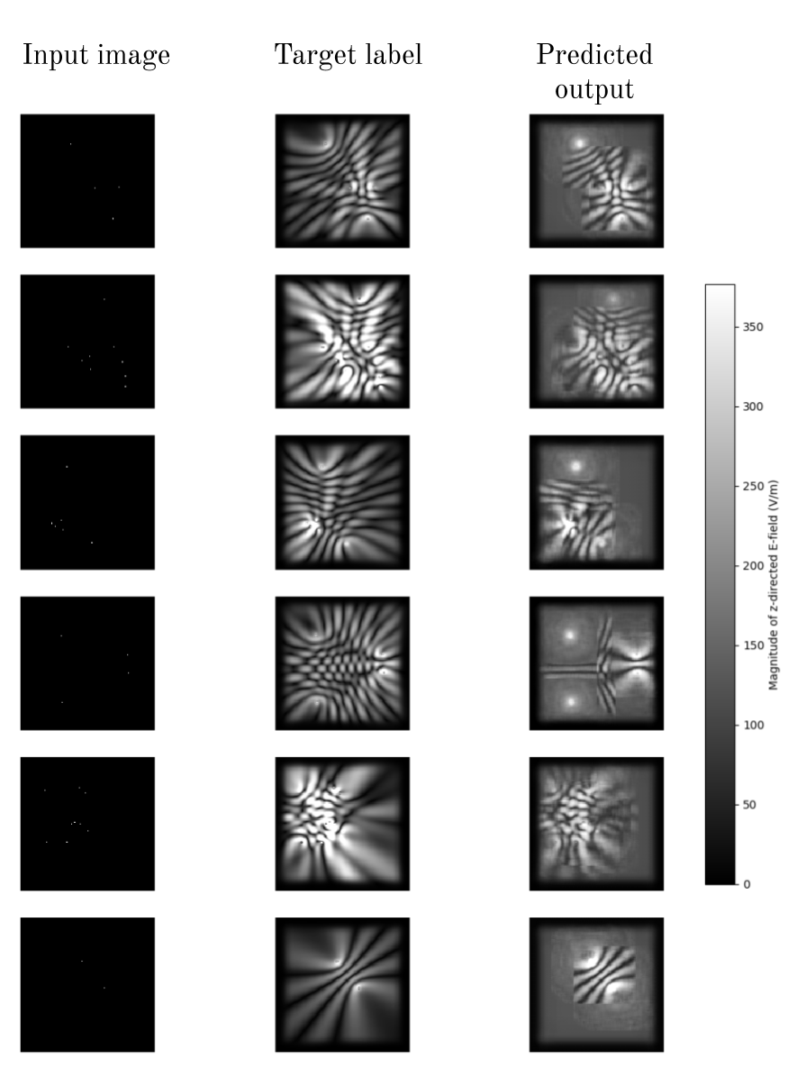
PS: this visual is easy to generate with the show_results() function mentioned earlier.

Again, after training for a while, substantial parts of each image unseen during training are predicted correctly, but seemingly in rectangular patches that look like they have been ‘pasted’ into the predicted image, and outside these rectangles the network appears to just give up and say “I have no idea what’s going on here, so let me be safe and rather just predict a \(1/r^2\) brightness from each source”.

To keep things grounded, remember that the input image has white pixels where a Hertzian dipole exists, and the output is the H-plane \(|E_z|\) of the antenna array, using the scale shown. The antenna array is an array of z-directed Hertzian dipoles lying in the xy plane.

Speed improvements

The worse accuracy comes at a much, much greater speed, which was one of the key goals of using a neural network approach. MEEP took quite a variable amount of time for each simulation, ranging from 3 seconds to 18 seconds for ones with more antenna elements. With proper optimization (symmetry mirrors, tuning optimizer settings) for each one, I’d imagine it could be boiled down to about 1.5s or even 1.2s.

Using the neural network approach, however, gives us a constant simulation time for a given simulation cell size. In particular, the resnet34 based UNet could produce predictions in 125ms-140ms. This is massive speedup from the MEEP frequency-domain solver, and could foreseeably also be sped up by computing predctions in batches or pruning and optimizing the network (e.g. fp16 inference). In any event, the neural network takes less than a tenth of the time the MEEP simulator takes, and operates fast enough to render about 10 frames per second for a constantly changing simulation cell. This speedup is the primary benefit of using the neural network approach.

Note: the prediction speeds of the UNet are dependent on the hardware used. For this experiment, both the MEEP simulations and UNets were run on Google Colab’s notebook instances (with an attached GPU).

Conclusion and possible future expansions

Overall, the exercise was an interesting first step into seeing whether neural networks can predict electromagnetic fields. And when using a decent GPU, this prediction is well under a second and constant no matter how many sources are in the simulation cell – significantly faster than using MEEP or FEKO in a lot of cases.

The accuracy of the UNets, however, is not the best and varies quite a lot between unseen examples. With that said, the areas of the output where it predicts a distinct field pattern do indeed match the simulated values quite closely, and would appear to be a quite useful first approximation. One can imagine dragging around an antenna element in real time and observing how (an approximation of) the field changes, or even programmatically optimizing the location of antenna elements to achieve a desired field pattern. This could be done in a similar way to how adversarial examples are created for classification neural networks.

But let me get concrete. The experiment here was partially successful, where I note:

• The UNets accuracy in predicting the fields was not quite as good as I would have hoped.
• The speedup from using the UNets over simulation software was actually a bit more than I expected.
• The phenomenon of the neural network seeming to ‘stitch’ parts of field patterns together to make a final prediction was really unexpected, and I am still not quite certian how to modify, expand, or remove this behavior.

Although the results I achieved are not all to spectacular, they give me various ideas that might drastically improve the outputs, and take a further step toward the final goal of being able to find the 3D E and H fields for arbitrary 3D current distributions in arbitrary media. Specifically,

• The data was severely limited to 1000 images/examples (20% of which make up a validation set). But data generation is largely free, only requiring compute time. It would be really interesting to see how this fares with 10 000, or even 100 000 images and see what happens with the larger models.
  • I wanted to try this, but most electromagnetic simulation software packages cost tons of money, and having them be scriptable is pretty important. My hardware is super limited, so training time for the neural networks and simulation with MEEP (which still does not support windows :/) was done entirely on Colab. But for a first step 1000 images isn’t too horrible.
• Changing how the images are formed to allow more transformations. As mentioned earlier, cropping out the PML portion of each image would allow for each image to be rotated (kind-of) for data augmentation while training, which could diversify the data a lot. However, this also will need careful attention since the rotated image is still represented in a horizontal rectangle, and we don’t want the missing pixels to be just blank or mirrored from the inner field patterns…
• Another way to represent the images better for the network might be to instead of encoding the input image as one-hot for current sources, include a reasonably sized (1-2% of full image) blob of white centered on each source. I Think this might just help the network to recognize the source better when weird transforms like resizing and convolutions are applied.
  • Or even overlay (on top of the input image) a brightness proportional to \(\frac{1}{r}\) from each source, again just to help the network remember to account for the effect of sources far away from the source location.
• Explore more into the architecture and the whole receptive field argument, and see if using a different architecture with more simple convolutions perhaps allows the network to model the sources interacting with one another better.
• Perhaps even a different loss function is better suited when predicting EM fields (as opposed to the simple MSE loss I used). Since the field patterns include a lot of rapidly changing regions of bright/dark, the MSE loss might be coercing the network a bit too much to just predict its whole \(1/r\) brightness thing which we see in some of the predictions. There might be a better loss function which more gently penalizes it if the radiation pattern is slightly shifted from the correct one, as opposed to MSE which would severely penalize such an error since the incorrect bright regions would overlap the correct dark regions.

And finally, some more far fetched ideas for how this can be expanded to take some more steps toward the final goal:

• Allow arbitrary source magnitudes by simply making the brightness in the input image correspond to the magnitude of the source (however normalization for large sources becomes interesting…).
• Allow arbitrary source phases by adding a channel to the input image (which is currently just broadcast to the 3 input channels of each UNet) which represents the phase of each source at that source’s location. For example, the brightness in this channel at each pixel where a source is present could be proportional to the tangent of the source’s phase.
• Allow arbitrary simple media by adding a 3rd channel to the input which just encodes the relative permittivity of each pixel in the simulation cell. Another channel could be added for permeability, and even another for the imaginary part of the permittivity/permeability (to model lossy media).
• Try to use build a 3D Unet, to take in a 4D input tensor (3 spatial dimensions, one other for each feature channel), and use the same setup with a channel for source magnitude, phase, media… And then predict the full 3D output E and H fields at all points in space as a 4D tensor again (with 6 output channels, 3 for each spatial component of each vector field).

And as always, if you have any questions, are interested in some aspect I haven’t fully explained, or just have some ideas on how to take it further, please get in contact with me under the ‘About’ page. Thanks for your time!

Source code

If you are interested in checking out the code, reproducing the results, or expanding upon them, the code is available on Github. The code consists of two python notebooks:

1. A data generation notebook, which uses MEEP to generate the training/validation data. Link here
2. A training notebook, which uses Fastai v2 to train the UNets and view the results. Link here

Both should work if you run them directly in google Colab :). Watch out for compatibility issues with Pillow v7.x (at least for a month or two after this post’s release).